User:Tohline/SSC/Stability/BiPolytropes
Marginally Unstable (nc,ne) = (5,1) Bipolytropes

|
|---|
| | Tiled Menu | Tables of Content | Banner Video | Tohline Home Page | |
Overview
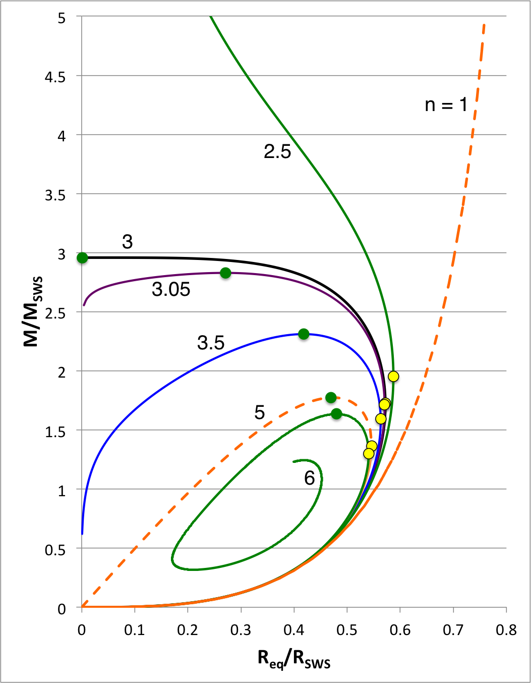
| Figure 1: Equilibrium Sequences of Pressure-Truncated Polytropes |
|---|
We expect the content of this chapter — which examines the relative stability of bipolytropes — to parallel in many ways the content of an accompanying chapter in which we have successfully analyzed the relative stability of pressure-truncated polytopes. Figure 1, shown here on the right, has been copied from a closely related discussion. The curves show the mass-radius relationship for pressure-truncated model sequences having a variety of polytropic indexes, as labeled, over the range <math>1 \le n \le 6</math>. (Another version of this figure includes the isothermal sequence.) On each sequence for which <math>~n \ge 3</math>, the green filled circle identifies the model with the largest mass. We have shown analytically that the oscillation frequency of the fundamental-mode of radial oscillation is precisely zero† for each one of these maximum-mass models. As a consequence, we know that each green circular marker identifies the point along its associated sequence that separates dynamically stable (larger radii) from dynamically unstable (smaller radii) models.
†In each case, the fundamental-mode oscillation frequency is precisely zero if, and only if, the adiabatic index governing expansions/contractions is related to the underlying structural polytropic index via the relation, <math>~\gamma_g = (n + 1)/n</math>, and if a constant surface-pressure boundary condition is imposed.
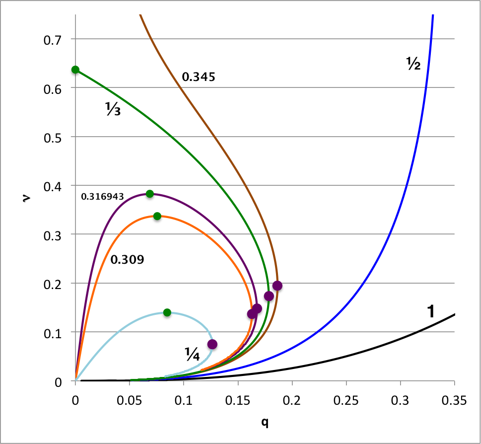
In another accompanying chapter, we have used purely analytic techniques to construct equilibrium sequences of spherically symmetric bipolytropes that have, <math>~(n_c,n_e) = (5,1)</math>. For a given choice of <math>~\mu_e/\mu_c</math> — the ratio of the mean-molecular weight of envelope material to the mean-molecular weight of material in the core — a physically relevant sequence of models can be constructed by steadily increasing the value of the dimensionless radius at the core/envelope interface, <math>~\xi_i</math>, from zero to infinity. Figure 2, whose content is essentially the same as Figure 1 of this separate chapter, shows how the fractional core mass, <math>\nu \equiv M_\mathrm{core}/M_\mathrm{tot}</math>, varies with the fractional core radius, <math>q \equiv r_\mathrm{core}/R</math>, along sequences having seven different values of <math>~\mu_e/\mu_c</math>, as labeled: 1 (black), ½ (dark blue), 0.345 (brown), ⅓ (dark green), 0.316943 (purple), 0.309 (orange), and ¼ (light blue).
When modeling bipolytropes, the default expectation is that an increase in <math>~\xi_i</math> along a given sequence will correspond to an increase in the relative size — both the radius and the mass — of the core. This expectation is realized along the Figure 2 sequences that have the largest mean-molecular weight ratios: <math>~\mu_e/\mu_c</math> = 1 and ½. But the behavior is different along the other five illustrated sequences. For sufficiently large <math>~\xi_i</math>, the relative radius of the core begins to decrease; along each sequence, a solid purple circular marker identifies the location of this turning point in radius. Furthermore, along sequences for which <math>~\mu_e/\mu_c < \tfrac{1}{3}</math>, eventually the fractional mass of the core reaches a maximum and, thereafter, decreases even as the value of <math>~\xi_i</math> continues to increase; a solid green circular marker identifies the location of this maximum mass turning point along each of these sequences. (Additional properties of these equilibrium sequences are discussed in yet another accompanying chapter.)
The principal question is: Along bipolytropic sequences, are maximum-mass models associated with the onset of dynamical instabilities?
Planned Approach
| Figure 2: Equilibrium Sequences of Bipolytropes with <math>~(n_c,n_e) = (5,1)</math> and Various <math>~\mu_e/\mu_c</math> |
|
|---|---|
Ideally we would like to answer the just-stated "principal question" using purely analytic techniques. But, to date, we have been unable to fully address the relevant issues analytically, even in what would be expected to be the simplest case: bipolytropic models that have <math>~(n_c,n_e) = (0, 0)</math>. Instead, we will streamline the investigation a bit and proceed — at least initially — using a blend of techniques. We will investigate the relative stability of bipolytropic models having <math>~(n_c,n_e) = (5,1) </math> whose equilibrium structures are completely defined analytically; then the eigenvectors describing radial modes of oscillation will be determined, one at a time, by solving the relevant LAWE(s) numerically. We are optimistic that this can be successfully accomplished because we have had experience numerically integrating the LAWE that governs the oscillation of:
- Isolated n = 3 polytropes — including a quantitative comparison against Schwarzschild's (1941) published work;
- Pressure-truncated isothermal spheres — including a quantitative comparison against the published analysis of Taff & Van Horn (1974); and
- Pressure-truncated n = 5 polytropes.
A key reference throughout this investigation will be the paper by J. O. Murphy & R. Fiedler (1985b, Proc. Astr. Soc. of Australia, 6, 222). They studied Radial Pulsations and Vibrational Stability of a Sequence of Two Zone Polytropic Stellar Models. Specifically, their underlying equilibrium models were bipolytropes that have <math>~(n_c,n_e) = (1, 5)</math>. In an accompanying chapter, we describe in detail how Murphy & Fiedler obtained these equilibrium bipolytropic structures and detail some of their equilibrium properties.
Here are the steps we initially plan to take:
- Governing LAWEs:
- Identify the relevant LAWEs that govern the behavior of radial oscillations in the <math>~n_c = 5</math> core and, separately, in the <math>~n_e = 1</math> envelope. Check these LAWE specifications against the published work of Murphy & Fiedler (1985b).
- Determine the matching conditions that must be satisfied across the core/envelope interface. Be sure to take into account the critical interface jump conditions spelled out by P. Ledoux & Th. Walraven (1958), as we have already discussed in the context of an analysis of radial oscillations in zero-zero bipolytropes.
- Determine what surface boundary condition should be imposed on physically relevant LAWE solutions, i.e., on the physically relevant radial-oscillation eigenvectors.
- Initial Analysis:
- Choose a maximum-mass model along the bipolytropic sequence that has, for example, <math>~\mu_e/\mu_c = 1/4</math>. Hopefully, we will be able to identify precisely (analytically) where this maximum-mass model lies along the sequence. Yes! Our earlier analysis does provide an analytic prescription of the model that sits at the maximum-mass location along the chosen sequence.
- Solve the relevant eigenvalue problem for this specific model, initially for <math>~(\gamma_c, \gamma_e) = (6/5, 2)</math> and initially for the fundamental mode of oscillation.
Virial Analysis
In an accompanying chapter we have examined the viral stability of <math>~(n_c, n_e) = (5, 1)</math> bipolytropes — see also an associated discussion of the free-energy of these configurations. We present, here, an overview of this separate discussion in an effort to provide a broader perspective to the focus of this current chapter.
Various Energy Expressions
Drawing from our accompanying detailed discussion, we have,
|
<math>~\mathfrak{G}</math> |
<math>~=</math> |
<math>~W_\mathrm{grav}\biggr|_\mathrm{core} + \mathfrak{S}_A\biggr|_\mathrm{core} + W_\mathrm{grav}\biggr|_\mathrm{env} + \mathfrak{S}_A\biggr|_\mathrm{env} </math> |
|
|
<math>~=</math> |
<math> ~W_\mathrm{grav}\biggr|_\mathrm{core} + \biggl[ \frac{2}{3(\gamma_c - 1)} \biggr] S_\mathrm{core} + W_\mathrm{grav}\biggr|_\mathrm{env} + \biggl[ \frac{2}{3(\gamma_e - 1)} \biggr] S_\mathrm{env} \, . </math> |
Recognizing that,
|
<math>~q</math> |
<math>~\equiv</math> |
<math>~\frac{r_i}{R} = \frac{\eta_i}{\eta_s} \, ,</math> |
|
<math>~\nu</math> |
<math>~\equiv</math> |
<math>~\frac{M_\mathrm{core}}{M_\mathrm{tot}} \, ,</math> |
|
<math>~\ell</math> |
<math>~\equiv</math> |
<math>~\frac{\xi}{\sqrt{3}} \, ,</math> |
|
<math>~\chi_\mathrm{eq} </math> |
<math>~=</math> |
<math>~\biggl( \frac{\pi}{2^3 \cdot 3^6}\biggr)^{1 / 2} \biggl( \frac{\nu}{q^3} \biggr)^{2} \biggl( 1 + \ell_i^2 \biggr)^{3} \biggl( \frac{q}{\ell_i}\biggr)^{5 } \, , </math> |
we have,
|
<math>~- \chi \biggl[ \frac{W_\mathrm{grav}}{E_\mathrm{norm}} \biggr]_\mathrm{core}</math> |
<math>~=</math> |
<math> \biggl[\biggl(\frac{3}{2^4}\biggr) \biggl( \frac{q}{\ell_i}\biggr)^{5}\biggl(\frac{\nu}{q^3} \biggr)^2 \biggl( 1 + \ell_i^2 \biggr)^{3} \biggr]_\mathrm{eq} \biggl[ \ell_i (\ell_i^4 - \frac{8}{3}\ell_i^2 - 1) (\ell_i^2 +1)^{-3} + \tan^{-1}\ell_i \biggr] </math> |
|
<math>~\Rightarrow ~~~ \biggl[ \frac{W_\mathrm{grav}}{E_\mathrm{norm}} \biggr]_\mathrm{core}</math> |
<math>~=</math> |
<math>- \frac{\chi_\mathrm{eq}}{\chi} \biggl( \frac{3^8}{2^5 \pi}\biggr)^{1 / 2} \biggl[ \ell_i (\ell_i^4 - \frac{8}{3}\ell_i^2 - 1) (\ell_i^2 +1)^{-3} + \tan^{-1}\ell_i \biggr] \, . </math> |
Next, given that,
|
<math>~b_\eta = \eta_s</math> |
and |
<math>~b_\eta q = \eta_i = 3\biggl( \frac{\mu_e}{\mu_c} \biggr) \ell_i (1 + \ell_i^2)^{-1} \, ,</math> |
we have,
|
<math>~\biggl[ \frac{W_\mathrm{grav}}{E_\mathrm{norm}} \biggr]_\mathrm{env}</math> |
<math>~=</math> |
<math> - \frac{\chi_\mathrm{eq}}{\chi} \biggl( \frac{\mu_e}{\mu_c} \biggr)^{-3} \biggl( \frac{1}{2^3\pi} \biggr)^{1/2} A^2 \biggl[6 b_\eta x - 3\sin[2(b_\eta x-B)] - 4b_\eta x \sin^2(b_\eta x - B) \biggr]_q^1 </math> |
|
|
<math>~=</math> |
<math> - \frac{\chi_\mathrm{eq}}{\chi} \biggl( \frac{\mu_e}{\mu_c} \biggr)^{-3} \biggl( \frac{1}{2^3\pi} \biggr)^{1/2} A^2 \biggl\{ \biggl[ 6 \eta_s - 3\sin[2(\eta_s -B)] - 4\eta_s \sin^2(\eta_s - B) \biggr] - \biggl[ 6 \eta_i - 3\sin[2(\eta_i -B)] - 4\eta_i \sin^2(\eta_i - B) \biggr] \biggr\} \, . </math> |
Also, given that,
|
<math>~q a_\xi^{1 / 2}</math> |
<math>~=</math> |
<math>~\frac{\xi_i}{\sqrt{3}} \, ,</math> |
we have,
|
<math>~\biggl( \frac{\mathfrak{S}_A}{E_\mathrm{norm}} \biggr)_\mathrm{core}</math> |
<math>~=</math> |
<math> \frac{2}{3({\gamma_c}-1)} \biggl( \frac{\chi}{\chi_\mathrm{eq}} \biggr)^{3-3\gamma_c} \biggl\{\biggl( \frac{3^8}{2^7\pi} \biggr)^{1/2} \biggl[ \tan^{-1}[a_\xi^{1/2}q] - a_\xi^{1/2}q ~\frac{(1 - a_\xi q^2)}{(1 + a_\xi q^2)^2} \biggr] \biggr\} </math> |
|
|
<math>~=</math> |
<math> \frac{2}{3({\gamma_c}-1)} \biggl( \frac{\chi}{\chi_\mathrm{eq}} \biggr)^{3-3\gamma_c} \biggl\{\biggl( \frac{3^8}{2^7\pi} \biggr)^{1/2} \biggl[ \tan^{-1}\biggl( \frac{\xi_i}{\sqrt{3}}\biggr) - \biggl( \frac{\xi_i}{\sqrt{3}}\biggr)\frac{(1 - \xi_i^2/3)}{(1 + \xi_i^2/3)^2} \biggr] \biggr\} </math> |
Finally, then, we can write,
|
<math>~\biggl( \frac{\mathfrak{S}_A}{E_\mathrm{norm}} \biggr)_\mathrm{env}</math> |
<math>~=</math> |
<math> \frac{2}{3({\gamma_e}-1)} \biggl( \frac{\chi}{\chi_\mathrm{eq}} \biggr)^{3-3\gamma_e} \biggl\{ \biggl( \frac{\mu_e}{\mu_c} \biggr)^{-3} A^2 \biggl( \frac{3^2}{2^5\pi} \biggr)^{1/2} \biggl[ 2b_\eta x -\sin[2(b_\eta x - B)] \biggr]_q^1 \biggr\} </math> |
|
|
|
<math>~=</math> |
<math> \frac{2}{3({\gamma_e}-1)} \biggl( \frac{\chi}{\chi_\mathrm{eq}} \biggr)^{3-3\gamma_e} \bigg( \frac{\mu_e}{\mu_c} \biggr)^{-3} A^2 \biggl( \frac{3^2}{2^5\pi} \biggr)^{1/2} \biggl\{ \biggl[ 2\eta_s -\sin[2(\eta_s - B)] \biggr] - \biggl[ 2\eta_i -\sin[2(\eta_i - B)] \biggr] \biggr\} \ . </math> |
Free Energy and Its Derivatives
We can now rewrite the free-energy expression in the form,
|
<math>~\mathfrak{g} \equiv \frac{\mathfrak{G}}{E_\mathrm{norm}}</math> |
<math>~=</math> |
<math> ~-\biggl(\frac{\chi_\mathrm{eq}}{\chi}\biggr)\mathfrak{w} + \biggl[ \frac{2}{3(\gamma_c - 1)} \biggr] \biggl(\frac{\chi}{\chi_\mathrm{eq}}\biggr)^{3 - 3\gamma_c}\mathfrak{s}_\mathrm{core} + \biggl[ \frac{2}{3(\gamma_e - 1)} \biggr] \biggl(\frac{\chi}{\chi_\mathrm{eq}}\biggr)^{3 - 3\gamma_e}\mathfrak{s}_\mathrm{env} \, , </math> |
where,
|
<math>~\mathfrak{s}_\mathrm{core}</math> |
<math>~\equiv</math> |
<math>~ \biggl( \frac{3^8}{2^7\pi} \biggr)^{1/2} \biggl[ \tan^{-1}\biggl( \frac{\xi_i}{\sqrt{3}}\biggr) - \biggl( \frac{\xi_i}{\sqrt{3}}\biggr)\frac{(1 - \xi_i^2/3)}{(1 + \xi_i^2/3)^2} \biggr]\, , </math> |
|
<math>~\mathfrak{s}_\mathrm{env}</math> |
<math>~\equiv</math> |
<math>~ \bigg( \frac{\mu_e}{\mu_c} \biggr)^{-3} A^2 \biggl( \frac{3^2}{2^5\pi} \biggr)^{1/2} \biggl\{ \biggl[ 2\eta_s -\sin[2(\eta_s - B)] \biggr] - \biggl[ 2\eta_i -\sin[2(\eta_i - B)] \biggr] \biggr\} \, , </math> |
|
<math>~\mathfrak{w}</math> |
<math>~\equiv</math> |
<math>~ \biggl( \frac{3^8}{2^5 \pi}\biggr)^{1 / 2} \biggl[ \ell_i (\ell_i^4 - \frac{8}{3}\ell_i^2 - 1) (\ell_i^2 +1)^{-3} + \tan^{-1}\ell_i \biggr] </math> |
|
|
|
<math>~ +~ \biggl( \frac{\mu_e}{\mu_c} \biggr)^{-3} \biggl( \frac{1}{2^3\pi} \biggr)^{1/2} A^2 \biggl\{ \biggl[ 6 \eta_s - 3\sin[2(\eta_s -B)] - 4\eta_s \sin^2(\eta_s - B) \biggr] - \biggl[ 6 \eta_i - 3\sin[2(\eta_i -B)] - 4\eta_i \sin^2(\eta_i - B) \biggr] \biggr\} \, . </math> |
The first derivative is,
|
<math>~\frac{d\mathfrak{g}}{d\chi} </math> |
<math>~=</math> |
<math> +~\biggl(\frac{\chi_\mathrm{eq}}{\chi^2}\biggr)\mathfrak{w} ~-~\frac{2}{\chi_\mathrm{eq}} \biggl[\biggl(\frac{\chi}{\chi_\mathrm{eq}}\biggr)^{2 - 3\gamma_c}\mathfrak{s}_\mathrm{core} ~+~\biggl(\frac{\chi}{\chi_\mathrm{eq}}\biggr)^{2 - 3\gamma_e}\mathfrak{s}_\mathrm{env} \biggr] \, . </math> |
And the second derivative is,
|
<math>~\frac{d^2\mathfrak{g}}{d\chi^2} </math> |
<math>~=</math> |
<math> -~2\biggl(\frac{\chi_\mathrm{eq}}{\chi^3}\biggr)\mathfrak{w} ~-~\frac{2}{\chi_\mathrm{eq}^2} \biggl[(2 - 3\gamma_c) \biggl(\frac{\chi}{\chi_\mathrm{eq}}\biggr)^{1 - 3\gamma_c}\mathfrak{s}_\mathrm{core} ~+~(2 - 3\gamma_e)\biggl(\frac{\chi}{\chi_\mathrm{eq}}\biggr)^{1 - 3\gamma_e}\mathfrak{s}_\mathrm{env} \biggr] \ . </math> |
What to Expect for Equilibrium Configurations
In equilibrium we should set <math>~d\mathfrak{g}/d\chi = 0</math> and <math>~\chi = \chi_\mathrm{eq}</math>. In which case we should expect to find that,
|
<math>~0 </math> |
<math>~=</math> |
<math> \frac{1}{\chi_\mathrm{eq}}\biggl[\mathfrak{w} ~-~2(\mathfrak{s}_\mathrm{core} ~+~\mathfrak{s}_\mathrm{env}) \biggr] \, . </math> |
In addition, an evaluation of the second derivative should give,
|
<math>~\frac{\chi_\mathrm{eq}^2}{2} \cdot \frac{d^2\mathfrak{g}}{d\chi^2} </math> |
<math>~=</math> |
<math> -~\mathfrak{w} ~-~ \biggl[(2 - 3\gamma_c) \mathfrak{s}_\mathrm{core} ~+~(2 - 3\gamma_e)\mathfrak{s}_\mathrm{env} \biggr] \, . </math> |
Then, the transition from stable to unstable configurations occurs when <math>~d^2\mathfrak{g}/d\chi^2 = 0</math>, that is, when,
|
<math>~\mathfrak{w} </math> |
<math>~=</math> |
<math> ~-~ \biggl[(2 - 3\gamma_c) \mathfrak{s}_\mathrm{core} ~+~(2 - 3\gamma_e)\mathfrak{s}_\mathrm{env} \biggr] </math> |
|
<math>~\Rightarrow ~~~0</math> |
<math>~=</math> |
<math> ~(4 - 3\gamma_c) \mathfrak{s}_\mathrm{core} ~+~(4 - 3\gamma_e)\mathfrak{s}_\mathrm{env} </math> |
|
<math>~\Rightarrow ~~~\frac{\mathfrak{s}_\mathrm{core} }{\mathfrak{s}_\mathrm{env}} </math> |
<math>~=</math> |
<math> ~-~\frac{(4 - 3\gamma_e) }{(4 - 3\gamma_c) } \, . </math> |
For example, if we set <math>~\gamma_c = 6/5</math> and <math>~\gamma_e = 2</math>, this implies,
|
<math>~\frac{\mathfrak{s}_\mathrm{core} }{\mathfrak{s}_\mathrm{env}} </math> |
<math>~=</math> |
<math> ~\frac{2 }{(4 - 18/5) } = 5 \, . </math> |
Virial Stability Evaluation
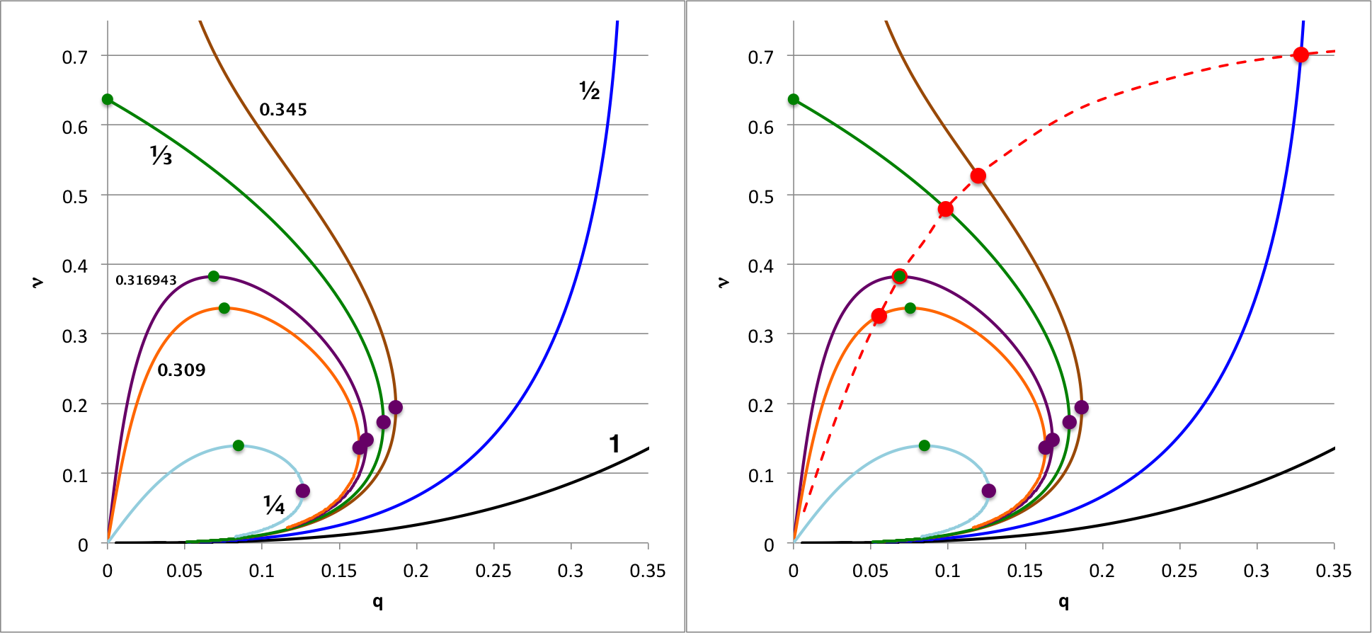
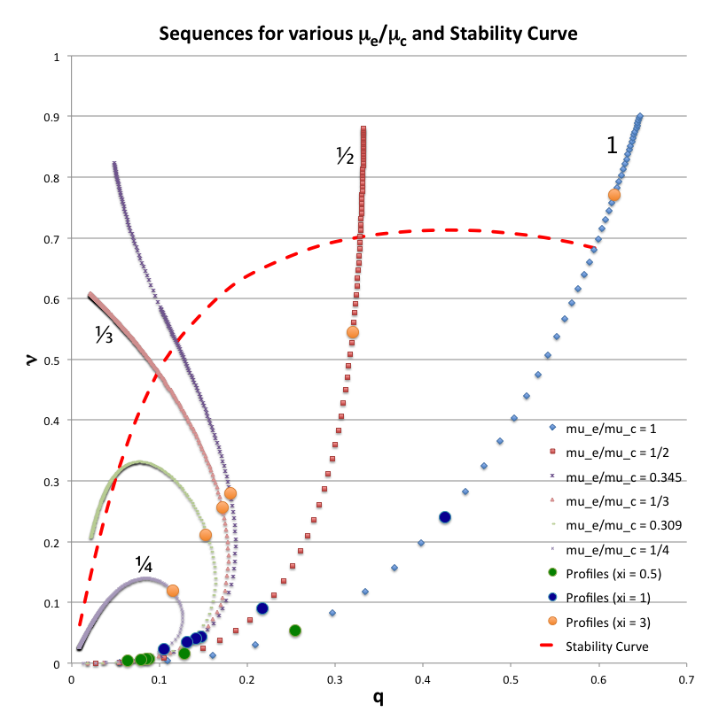
The left-hand panel of Figure 3 is identical to Figure 2, above. It displays in the <math>~q-\nu</math> parameter space, the behavior of <math>~(n_c, n_e) = (5, 1)</math> bipolytropic equilibrium sequences that have, as labeled, seven different values of the ratio of mean-molecular-weights, <math>~\mu_e/\mu_c</math>. Using a numerical root-finding technique, we have determined where the virial stability condition, <math>~\mathfrak{s}_\mathrm{core}/\mathfrak{s}_\mathrm{env} = 5</math>, is satisfied along each of these sequences — as well as along a number of additional equilibrium sequences. Key properties of each of these identified models have been recorded in Table 1 of an accompanying discussion; see also an associated discussion of the free-energy of these configurations. Pulling from this tabulated data, the solid-red circular markers that appear in the right-hand panel of Figure 3 identify where this virial stability condition is satisfied along the separate equilibrium sequences while the accompanying dashed red curve identifies more broadly how the <math>~q-\nu</math> parameter space is divided into stable (below and to the right) versus unstable (above and to the left) regions.
| Figure 3 |
|---|
In what follows we use a complementary — and more quantitatively rigorous — approach to evaluating the stability of equilibrium models, and contrast the results of that analysis with the virial-analysis results presented graphically here in Figure 3.
Review of the Analysis by Murphy & Fiedler (1985b)
As we have detailed separately, the boundary condition at the center of a polytropic configuration is,
<math>~\frac{dx}{d\xi} \biggr|_{\xi=0} = 0 \, ;</math>
and the boundary condition at the surface of an isolated polytropic configuration is,
|
<math>~\frac{d\ln x}{d\ln\xi}</math> |
<math>~=</math> |
<math>~- \alpha + \frac{\omega^2}{\gamma_g } \biggl( \frac{1}{4\pi G \rho_c } \biggr) \frac{\xi}{(-\theta^')} </math> at <math>~\xi = \xi_s \, .</math> |
But this surface condition is not applicable to bipolytropes. Instead, let's return to the original, more general expression of the surface boundary condition:
|
<math>~ \frac{d\ln x}{d\ln\xi}\biggr|_s</math> |
<math>~=</math> |
<math>~- \alpha + \frac{\omega^2 R^3}{\gamma_g GM_\mathrm{tot}} \, .</math> |
|
Utilizing an accompanying discussion, let's examine the frequency normalization used by Murphy & Fiedler (1985b) (see the top of the left-hand column on p. 223):
For a given radial quantum number, <math>~k</math>, the factor inside the square brackets in this last expression is what Murphy & Fiedler (1985b) refer to as <math>~\omega^2_k \theta_c</math>. Keep in mind, as well, that, in the notation we are using,
This also means that the surface boundary condition may be rewritten as,
|
Let's apply these relations to the core and envelope, separately.
Interface Conditions
Here, we will simply copy the discussion already provided in the context of our attempt to analyze the stability of <math>~(n_c, n_e) = (0, 0)</math> bipolytropes; specifically, we will draw from STEP 4: in the Piecing Together subsection. Following the discussion in §§57 & 58 of P. Ledoux & Th. Walraven (1958), the proper treatment is to ensure that fractional perturbation in the gas pressure (see their equation 57.31),
|
<math>~\frac{\delta P}{P}</math> |
<math>~=</math> |
<math>~- \gamma x \biggl( 3 + \frac{d\ln x}{d\ln \xi} \biggr) \, ,</math> |
is continuous across the interface. That is to say, at the interface <math>~(\xi = \xi_i)</math>, we need to enforce the relation,
|
<math>~0</math> |
<math>~=</math> |
<math>~\biggl[ \gamma_c x_\mathrm{core} \biggl( 3 + \frac{d\ln x_\mathrm{core}}{d\ln \xi} \biggr) - \gamma_e x_\mathrm{env} \biggl( 3 + \frac{d\ln x_\mathrm{env}}{d\ln \xi} \biggr)\biggr]_{\xi=\xi_i}</math> |
|
|
<math>~=</math> |
<math>~\gamma_e \biggl[ \frac{\gamma_c}{\gamma_e} \biggl( 3 + \frac{d\ln x_\mathrm{core}}{d\ln \xi} \biggr) - \biggl( 3 + \frac{d\ln x_\mathrm{env}}{d\ln \xi} \biggr)\biggr]_{\xi=\xi_i}</math> |
|
<math>~\Rightarrow~~~ \frac{d\ln x_\mathrm{env}}{d\ln \xi} \biggr|_{\xi=\xi_i}</math> |
<math>~=</math> |
<math>~3\biggl(\frac{\gamma_c}{\gamma_e} -1\biggr) + \frac{\gamma_c}{\gamma_e} \biggl( \frac{d\ln x_\mathrm{core}}{d\ln \xi} \biggr)_{\xi=\xi_i} \, .</math> |
In the context of this interface-matching constraint (see their equation 62.1), P. Ledoux & Th. Walraven (1958) state the following: In the static (i.e., unperturbed equilibrium) model … discontinuities in <math>~\rho</math> or in <math>~\gamma</math> might occur at some [radius]. In the first case — that is, a discontinuity only in density, while <math>~\gamma_e = \gamma_c</math> — the interface conditions imply the continuity of <math>~\tfrac{1}{x} \cdot \tfrac{dx}{d\xi}</math> at that [radius]. In the second case — that is, a discontinuity in the adiabatic exponent — the dynamical condition may be written as above. This implies a discontinuity of the first derivative at any discontinuity of <math>~\gamma</math>.
The algorithm that Murphy & Fiedler (1985b) used to "… [integrate] through each zone …" was designed "… with continuity in <math>~x</math> and <math>~dx/d\xi</math> being imposed at the interface …" Given that they set <math>~\gamma_c = \gamma_e = 5/3</math>, their interface matching condition is consistent with the one prescribed by P. Ledoux & Th. Walraven (1958).
Radial Oscillations of (nc, ne) = (5, 1) Models
Foundation
In an accompanying discussion, we derived the so-called,
Adiabatic Wave (or Radial Pulsation) Equation
|
<math>~ \frac{d^2x}{dr_0^2} + \biggl[\frac{4}{r_0} - \biggl(\frac{g_0 \rho_0}{P_0}\biggr) \biggr] \frac{dx}{dr_0} + \biggl(\frac{\rho_0}{\gamma_\mathrm{g} P_0} \biggr)\biggl[\omega^2 + (4 - 3\gamma_\mathrm{g})\frac{g_0}{r_0} \biggr] x = 0 </math> |
whose solution gives eigenfunctions that describe various radial modes of oscillation in spherically symmetric, self-gravitating fluid configurations. Assuming that the underlying equilibrium structure is that of a bipolytrope having <math>~(n_c, n_e) = (5, 1)</math>, it makes sense to adopt the normalizations used when defining the equilibrium structure, namely,
|
<math>~\rho^*</math> |
<math>~\equiv</math> |
<math>~\frac{\rho_0}{\rho_c}</math> |
; |
<math>~r^*</math> |
<math>~\equiv</math> |
<math>~\frac{r_0}{[K_c^{1/2}/(G^{1/2}\rho_c^{2/5})]}</math> |
|
<math>~P^*</math> |
<math>~\equiv</math> |
<math>~\frac{P_0}{K_c\rho_c^{6/5}}</math> |
; |
<math>~M_r^*</math> |
<math>~\equiv</math> |
<math>~\frac{M_r}{[K_c^{3/2}/(G^{3/2}\rho_c^{1/5})]}</math> |
We note as well that,
|
<math>~g_0</math> |
<math>~=</math> |
<math>~\frac{GM(r_0)}{r_0^2}</math> |
|
|
<math>~=</math> |
<math>~ G \biggl[ M_r^* \rho_c^{-1 / 5} \biggl( \frac{K_c}{G}\biggr)^{3 / 2} \biggr] \biggl[ r^* \rho_c^{-2 / 5}\biggl( \frac{K_c}{G}\biggr)^{1 / 2} \biggr]^{-2} </math> |
|
|
<math>~=</math> |
<math>~ \frac{G M_r^*}{(r^*)^2} \biggl[ \rho_c^{3 / 5} \biggl( \frac{K_c}{G}\biggr)^{1 / 2} \biggr] \, . </math> |
Hence, multiplying the LAWE through by <math>~(K_c/G)\rho_c^{-4 / 5}</math> gives,
|
<math>~0</math> |
<math>~=</math> |
<math>~ \frac{d^2x}{dr_0^2} + \biggl[\frac{4}{r_0} - \biggl(\frac{g_0 \rho_0}{P_0}\biggr) \biggr] \frac{dx}{dr_0} + \biggl(\frac{\rho_0}{\gamma_\mathrm{g} P_0} \biggr)\biggl[\omega^2 + (4 - 3\gamma_\mathrm{g})\frac{g_0}{r_0} \biggr] x </math> |
|
<math>~0</math> |
<math>~=</math> |
<math>~ \frac{d^2x}{dr*^2} + \biggl[\frac{4}{r^*} ~-~ \rho_c^{-2 / 5} \biggl( \frac{K_c}{G} \biggr)^{1 / 2}\biggl(\frac{g_0 \rho_0}{P_0}\biggr) \biggr] \frac{dx}{dr*} ~+~ \rho_c^{-4 / 5}\biggl( \frac{K_c}{G} \biggr)\biggl(\frac{\rho_0}{\gamma_\mathrm{g} P_0} \biggr)\biggl[\omega^2 ~+~ (4 - 3\gamma_\mathrm{g})\frac{g_0}{r_0} \biggr] x </math> |
|
|
<math>~=</math> |
<math>~ \frac{d^2x}{dr*^2} ~+~ \biggl\{\frac{4}{r^*} ~-~ \rho_c^{-2 / 5} \biggl( \frac{K_c}{G} \biggr)^{1 / 2} \frac{G M_r^*}{(r^*)^2} \biggl[ \rho_c^{3 / 5} \biggl( \frac{K_c}{G}\biggr)^{1 / 2} \biggr] \biggl[ \frac{\rho_c \rho^*}{P^* K_c \rho_c^{6/5}}\biggr] \biggr\} \frac{dx}{dr*} ~+~ \rho_c^{-4 / 5}\biggl( \frac{K_c}{G} \biggr)\biggl[ \frac{\rho_c \rho^*}{\gamma_\mathrm{g}P^* K_c \rho_c^{6/5}}\biggr] \biggl\{\omega^2 ~+~ (4 - 3\gamma_\mathrm{g}) \frac{G M_r^*}{(r^*)^2} \biggl[ \rho_c^{3 / 5} \biggl( \frac{K_c}{G}\biggr)^{1 / 2} \biggr] \frac{\rho_c^{2 / 5}}{r^*}\biggl( \frac{G}{K_c}\biggr)^{1 / 2} \biggr\} x
</math> |
|
|
<math>~=</math> |
<math>~ \frac{d^2x}{dr*^2} ~+~ \biggl\{\frac{4}{r^*} ~-~ \frac{M_r^*}{(r^*)^2} \biggl[ \frac{\rho^*}{P^* }\biggr] \biggr\} \frac{dx}{dr*} ~+~ \biggl( \frac{1}{G\rho_c} \biggr)\biggl[ \frac{ \rho^*}{\gamma_\mathrm{g}P^* }\biggr] \biggl\{\omega^2 ~+~ (4 - 3\gamma_\mathrm{g}) \frac{G\rho_c M_r^*}{(r^*)^3} \biggr\} x
</math> |
|
|
<math>~=</math> |
<math>~ \frac{d^2x}{dr*^2} + \biggl\{ \frac{4}{r^*} -\biggl(\frac{\rho^*}{P^*}\biggr)\frac{ M_r^*}{(r^*)^2}\biggr\} \frac{dx}{dr*} + \biggl(\frac{\rho^*}{ P^* } \biggr)\biggl\{ \frac{\omega^2}{\gamma_\mathrm{g} G\rho_c} + \biggl(\frac{4}{\gamma_\mathrm{g}} - 3\biggr)\frac{ M_r^*}{(r^*)^3}\biggr\} x </math> |
|
|
<math>~=</math> |
<math>~ \frac{d^2x}{dr*^2} + \biggl\{ 4 -\biggl(\frac{\rho^*}{P^*}\biggr)\frac{ M_r^*}{(r^*)}\biggr\}\frac{1}{r^*} \frac{dx}{dr*} + \biggl(\frac{\rho^*}{ P^* } \biggr)\biggl\{ \frac{2\pi \sigma_c^2}{3\gamma_\mathrm{g}} ~-~\frac{\alpha_\mathrm{g} M_r^*}{(r^*)^3}\biggr\} x \, . </math> |
Profile
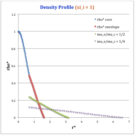
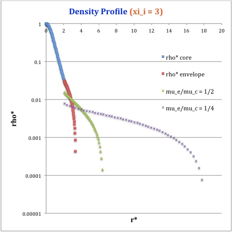
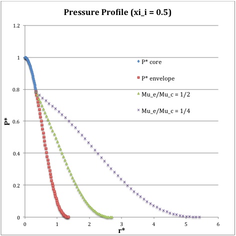
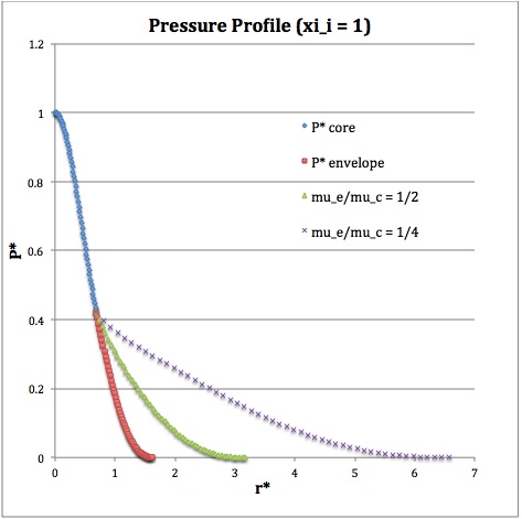
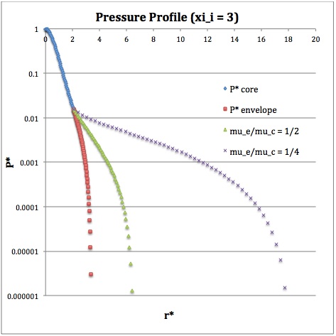
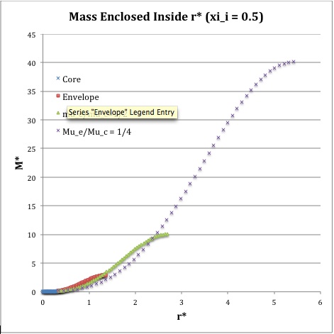
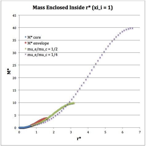
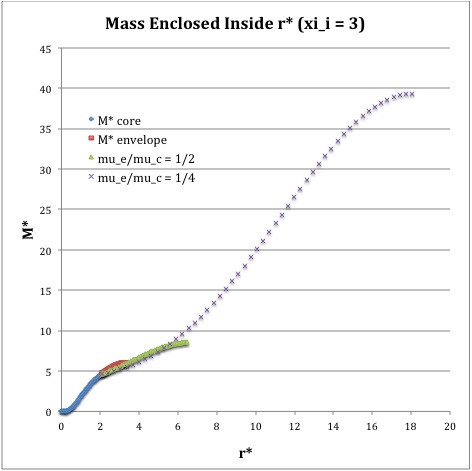
Now, referencing the derived bipolytropic model profile, we should incorporate the following relations:
Table 1: Radial Profile of Various Physical Variables
|
Variable |
Throughout the Core |
Throughout the Envelope† |
Plotted Profiles |
||
|
<math>~\xi_i = 0.5</math> |
<math>~\xi_i = 1.0</math> |
<math>~\xi_i = 3.0</math> |
|||
|
<math>~r^*</math> |
<math>\biggl( \frac{3}{2\pi} \biggr)^{1/2} \xi</math> |
<math>\biggl( \frac{\mu_e}{\mu_c} \biggr)^{-1} \theta^{-2}_i (2\pi)^{-1/2}\eta</math> |
|
||
|
<math>~\rho^*</math> |
<math>\biggl( 1 + \frac{1}{3}\xi^2 \biggr)^{-5/2}</math> |
<math>\biggl( \frac{\mu_e}{\mu_c} \biggr) \theta^{5}_i \phi(\eta)</math> |
|||
|
<math>~P^*</math> |
<math>\biggl( 1 + \frac{1}{3}\xi^2 \biggr)^{-3}</math> |
<math>\theta^{6}_i [\phi(\eta)]^{2}</math> |
|||
|
<math>~M_r^*</math> |
<math>\biggl( \frac{2\cdot 3}{\pi } \biggr)^{1/2} \biggl[ \xi^3 \biggl( 1 + \frac{1}{3}\xi^2 \biggr)^{-3/2} \biggr]</math> |
<math>\biggl( \frac{\mu_e}{\mu_c} \biggr)^{-2} \theta^{-1}_i \biggl( \frac{2}{\pi} \biggr)^{1/2} \biggl(-\eta^2 \frac{d\phi}{d\eta} \biggr)</math> |
|||
|
†In order to obtain the various envelope profiles, it is necessary to evaluate <math>\phi(\eta)</math> and its first derivative using the information presented in Step 6, above. |
|||||
Therefore, throughout the core we have,
|
<math>~\frac{\rho^*}{P^*}</math> |
<math>~=</math> |
<math>~\biggl( 1 + \frac{1}{3}\xi^2 \biggr)^{1 / 2} \, ;</math> |
|
<math>~\frac{M_r^*}{r^*}</math> |
<math>~=</math> |
<math>~ \biggl( \frac{2\cdot 3}{\pi } \biggr)^{1/2} \biggl[ \xi^3 \biggl( 1 + \frac{1}{3}\xi^2 \biggr)^{-3/2} \biggr]\biggl( \frac{2\pi}{3}\biggr)^{1 / 2} \frac{1}{\xi} = 2 \xi^2 \biggl( 1 + \frac{1}{3}\xi^2 \biggr)^{-3/2} \, ; </math> |
and, throughout the envelope we have,
|
<math>~\frac{\rho^*}{P^*}</math> |
<math>~=</math> |
<math>~ \biggl( \frac{\mu_e}{\mu_c} \biggr) \theta^{-1}_i \phi(\eta)^{-1} \, ; </math> |
|
<math>~\frac{M_r^*}{r^*}</math> |
<math>~=</math> |
<math>~ \biggl( \frac{\mu_e}{\mu_c} \biggr)^{-2} \theta^{-1}_i \biggl( \frac{2}{\pi} \biggr)^{1/2} \biggl(-\eta^2 \frac{d\phi}{d\eta} \biggr) \biggl[ \biggl( \frac{\mu_e}{\mu_c} \biggr)^{-1} \theta^{-2}_i (2\pi)^{-1/2}\eta \biggr]^{-1} = 2 \biggl( \frac{\mu_e}{\mu_c} \biggr)^{-1} \theta_i \eta \biggl(-\eta^2 \frac{d\phi}{d\eta} \biggr) \, . </math> |
Numerical Integration
General Approach
Here, we begin by recognizing that the 2nd-order ODE that must be integrated to obtain the desired eigenvectors has the generic form,
|
<math>~0</math> |
<math>~=</math> |
<math>~ x + \frac{\mathcal{H}}{r^*} x' + \mathcal{K}x \, , </math> |
where,
|
<math>~x'</math> |
<math>~=</math> |
<math>~\frac{dx}{dr^*}</math> |
and |
<math>~x</math> |
<math>~=</math> |
<math>~\frac{d^2x}{d(r^*)^2} \, .</math> |
Adopting the same approach as before when we integrated the LAWE for pressure-truncated polytropes, we will enlist the finite-difference approximations,
|
<math>~x'</math> |
<math>~\approx</math> |
<math>~ \frac{x_+ - x_-}{2\delta r^*} </math> |
and |
<math>~x</math> |
<math>~\approx</math> |
<math>~ \frac{x_+ -2x_j + x_-}{(\delta r^*)^2} \, . </math> |
The finite-difference representation of the LAWE is, therefore,
|
<math>~\frac{x_+ -2x_j + x_-}{(\delta r^*)^2}</math> |
<math>~=</math> |
<math>~ -~ \frac{\mathcal{H}}{r^*} \biggl[ \frac{x_+ - x_-}{2\delta r^*} \biggr] ~-~ \mathcal{K}x_j </math> |
|
<math>~\Rightarrow ~~~ x_+ -2x_j + x_-</math> |
<math>~=</math> |
<math>~ -~ \frac{\delta r^*}{2r^*} \biggl[ x_+ - x_- \biggr]\mathcal{H} ~-~ (\delta r^*)^2\mathcal{K}x_j </math> |
|
<math>~\Rightarrow ~~~ x_{j+1} \biggl[1 + \biggl( \frac{\delta r^*}{2r^*}\biggr) \mathcal{H} \biggr]</math> |
<math>~=</math> |
<math>~ \biggl[ 2 - (\delta r^*)^2\mathcal{K}\biggr] x_j ~-~\biggl[ 1 - \biggl( \frac{\delta r^*}{2r^*} \biggr) \mathcal{H} \biggr]x_{j-1} \, . </math> |
In what follows we will also find it useful to rewrite <math>~\mathcal{K}</math> in the form,
<math>~\mathcal{K} ~\rightarrow ~\biggl(\frac{\sigma_c^2}{\gamma_\mathrm{g}}\biggr) \mathcal{K}_1 - \alpha_\mathrm{g} \mathcal{K}_2 \, .</math>
The relevant coefficient expressions for all regions of the configuration are,
|
<math>~\mathcal{H}</math> |
<math>~\equiv</math> |
<math>~ \biggl\{ 4 -\biggl(\frac{\rho^*}{P^*}\biggr)\frac{ M_r^*}{(r^*)}\biggr\} </math> |
, |
<math>~\mathcal{K}_1</math> |
<math>~\equiv</math> |
<math>~ \frac{2\pi }{3}\biggl(\frac{\rho^*}{ P^* } \biggr) </math> |
and |
<math>~\mathcal{K}_2</math> |
<math>~\equiv</math> |
<math>~ \biggl(\frac{\rho^*}{ P^* } \biggr)\frac{M_r^*}{(r^*)^3} \, . </math> |
Special Handling at the Center
In order to kick-start the integration, we set the displacement function value to <math>~x_1 = 1</math> at the center of the configuration <math>~(\xi_1 = 0)</math>, then draw on the derived power-series expression to determine the value of the displacement function at the first radial grid line, <math>~\xi_2 = \delta\xi</math>, away from the center. Specifically, we set,
|
<math>~ x_2 </math> |
<math>~=</math> |
<math>~ x_1 \biggl[ 1 - \frac{(n+1) \mathfrak{F} (\delta\xi)^2}{60} \biggr]_{n=5} = x_1 \biggl[ 1 - \frac{\mathfrak{F} (\delta\xi)^2}{10} \biggr] \, .</math> |
Special Handling at the Interface
Integrating outward from the center, the general approach will work up through the determination of <math>~x_{j+1}</math> when "j+1" refers to the interface location. In order to properly transition from the core to the envelope, we need to determine the value of the slope at this interface location. Let's do this by setting j = i, then projecting forward to what <math>~x_+</math> would be — that is, to what the amplitude just beyond the interface would be — if the core were to be extended one more zone. Then, the slope at the interface (as viewed from the perspective of the core) will be,
|
<math>~x'_i\biggr|_\mathrm{core}</math> |
<math>~\approx</math> |
<math>~ \frac{1}{2\delta r^*} \biggl\{ x_+ - x_{i-1} \biggr\} </math> |
|
|
<math>~=</math> |
<math>~ -\frac{x_{i-1}}{2\delta r^*} + \frac{1}{2\delta r^*} \biggl\{ \biggl[ 2 - (\delta r^*)^2\mathcal{K}\biggr] x_i ~-~\biggl[ 1 - \biggl( \frac{\delta r^*}{2r^*} \biggr) \mathcal{H} \biggr]x_{i-1} \biggr\}\biggl[1 + \biggl( \frac{\delta r^*}{2r^*}\biggr) \mathcal{H} \biggr]^{-1} </math> |
|
|
<math>~=</math> |
<math>~ \frac{1}{2\delta r^*} \biggl\{ \biggl[ 2 - (\delta r^*)^2\mathcal{K}\biggr] x_i ~-~\biggl[ 1 - \biggl( \frac{\delta r^*}{2r^*} \biggr) \mathcal{H} \biggr]x_{i-1} ~-~\biggl[1 + \biggl( \frac{\delta r^*}{2r^*}\biggr) \mathcal{H} \biggr]x_{i-1} \biggr\}\biggl[1 + \biggl( \frac{\delta r^*}{2r^*}\biggr) \mathcal{H} \biggr]^{-1} </math> |
|
|
<math>~=</math> |
<math>~ \frac{1}{2\delta r^*} \biggl\{ \biggl[ 2 - (\delta r^*)^2\mathcal{K}\biggr] x_i ~-~2x_{i-1} \biggr\}\biggl[1 + \biggl( \frac{\delta r^*}{2r^*}\biggr) \mathcal{H} \biggr]^{-1} </math> |
Conversely, as viewed from the envelope, if we assume that we know <math>~x_i</math> and <math>~x'_i</math>, we can determine the amplitude, <math>~x_{i+1}</math>, at the first zone beyond the interface as follows:
|
<math>~x_-</math> |
<math>~\approx</math> |
<math>~ x_{i+1} - 2\delta r^*\cdot x'_i\biggr|_\mathrm{env} </math> |
|
<math>~\Rightarrow ~~~ x_{i+1} \biggl[1 + \biggl( \frac{\delta r^*}{2r^*}\biggr) \mathcal{H} \biggr]</math> |
<math>~=</math> |
<math>~ \biggl[ 2 - (\delta r^*)^2\mathcal{K}\biggr] x_i ~-~\biggl[ 1 - \biggl( \frac{\delta r^*}{2r^*} \biggr) \mathcal{H} \biggr] \biggl[ x_{i+1} - 2\delta r^*\cdot x'_i\biggr|_\mathrm{env} \biggr] </math> |
|
<math>~\Rightarrow ~~~ x_{i+1} \biggl[1 + \biggl( \frac{\delta r^*}{2r^*}\biggr) \mathcal{H} \biggr] ~+~ \biggl[ 1 - \biggl( \frac{\delta r^*}{2r^*} \biggr) \mathcal{H} \biggr] x_{i+1} </math> |
<math>~=</math> |
<math>~ \biggl[ 2 - (\delta r^*)^2\mathcal{K}\biggr] x_i ~+~ \biggl[ 1 - \biggl( \frac{\delta r^*}{2r^*} \biggr) \mathcal{H} \biggr] 2\delta r^*\cdot x'_i\biggr|_\mathrm{env} </math> |
|
<math>~\Rightarrow ~~~ x_{i+1} </math> |
<math>~=</math> |
<math>~ \biggl[ 1 - \tfrac{1}{2}(\delta r^*)^2\mathcal{K}\biggr] x_i ~+~ \biggl[ 1 - \biggl( \frac{\delta r^*}{2r^*} \biggr) \mathcal{H} \biggr] \delta r^*\cdot x'_i\biggr|_\mathrm{env} </math> |
Splitting Analysis Into Separate Core and Envelope Components
Core:
Given that, <math>~\sqrt{2\pi/3}~r^* = \xi</math>, lets multiply the LAWE through by <math>~3/(2\pi)</math>. This gives,
|
<math>~0</math> |
<math>~=</math> |
<math>~ \frac{d^2x}{d\xi^2} + \biggl\{ 4 -\biggl(\frac{\rho^*}{P^*}\biggr)\frac{ M_r^*}{(r^*)}\biggr\}\frac{1}{\xi} \cdot \frac{dx}{d\xi} + \frac{3}{2\pi}\biggl(\frac{\rho^*}{ P^* } \biggr)\biggl\{ \frac{2\pi \sigma_c^2}{3\gamma_\mathrm{g}} ~-~\frac{\alpha_\mathrm{g} M_r^*}{(r^*)^3}\biggr\} x \, . </math> |
Specifically for the core, therefore, the finite-difference representation of the LAWE is,
|
<math>~\frac{x_+ -2x_j + x_-}{(\delta \xi)^2}</math> |
<math>~=</math> |
<math>~ -~ \frac{\mathcal{H}}{\xi} \biggl[ \frac{x_+ - x_-}{2\delta \xi} \biggr] ~-~ \biggl[ \frac{3\mathcal{K}}{2\pi} \biggr]x_j </math> |
|
<math>~\Rightarrow ~~~ x_+ -2x_j + x_-</math> |
<math>~=</math> |
<math>~ -~ \frac{\delta \xi}{2\xi} \biggl[ x_+ - x_- \biggr]\mathcal{H} ~-~ (\delta \xi)^2 \biggl[ \frac{3\mathcal{K}}{2\pi} \biggr] x_j </math> |
|
<math>~\Rightarrow ~~~ x_{j+1} \biggl[1 + \biggl( \frac{\delta \xi}{2\xi}\biggr) \mathcal{H} \biggr]</math> |
<math>~=</math> |
<math>~ \biggl[ 2 - (\delta \xi)^2\biggl( \frac{3\mathcal{K}}{2\pi} \biggr) \biggr] x_j ~-~\biggl[ 1 - \biggl( \frac{\delta \xi}{2\xi} \biggr) \mathcal{H} \biggr]x_{j-1} \, . </math> |
This also means that, as viewed from the perspective of the core, the slope at the interface is
|
<math>~\biggl[ \frac{dx}{d\xi}\biggr]_\mathrm{interface}</math> |
<math>~=</math> |
<math>~ \frac{1}{2\delta \xi} \biggl\{ \biggl[ 2 - (\delta \xi)^2 \biggl( \frac{3\mathcal{K}}{2\pi} \biggr)\biggr] x_i ~-~2x_{i-1} \biggr\}\biggl[1 + \biggl( \frac{\delta \xi}{2\xi}\biggr) \mathcal{H} \biggr]^{-1} \, . </math> |
Envelope:
Given that,
<math>~\biggl( \frac{\mu_e}{\mu_c} \biggr) \theta_i^2 (2\pi)^{1 / 2}~r^* = \eta \, ,</math>
let's multiply the LAWE through by <math>~(2\pi)^{-1} \theta_i^{-4}( \mu_e/\mu_c)^{-2} </math>. This gives,
|
<math>~0</math> |
<math>~=</math> |
<math>~ \frac{d^2x}{d\eta^2} + \biggl\{ 4 -\biggl(\frac{\rho^*}{P^*}\biggr)\frac{ M_r^*}{(r^*)}\biggr\}\frac{1}{\eta} \cdot \frac{dx}{d\eta} + \frac{1}{2\pi \theta_i^4} \biggl( \frac{\mu_e}{\mu_c} \biggr)^{-2} \biggl(\frac{\rho^*}{ P^* } \biggr)\biggl\{ \frac{2\pi \sigma_c^2}{3\gamma_\mathrm{g}} ~-~\frac{\alpha_\mathrm{g} M_r^*}{(r^*)^3}\biggr\} x \, . </math> |
Specifically for the envelope, therefore, the finite-difference representation of the LAWE is,
|
<math>~\frac{x_+ -2x_j + x_-}{(\delta \eta)^2}</math> |
<math>~=</math> |
<math>~ -~ \frac{\mathcal{H}}{\eta} \biggl[ \frac{x_+ - x_-}{2\delta \eta} \biggr] ~-~ \biggl( \frac{\mu_e}{\mu_c} \biggr)^{-2}\biggl[ \frac{\mathcal{K}}{2\pi \theta_i^4} \biggr]x_j </math> |
|
<math>~\Rightarrow ~~~ x_+ -2x_j + x_-</math> |
<math>~=</math> |
<math>~ -~ \frac{\delta \eta}{2\eta} \biggl[ x_+ - x_- \biggr]\mathcal{H} ~-~ (\delta \eta)^2 \biggl( \frac{\mu_e}{\mu_c} \biggr)^{-2}\biggl[ \frac{\mathcal{K}}{2\pi \theta_i^4} \biggr] x_j </math> |
|
<math>~\Rightarrow ~~~ x_{j+1} \biggl[1 + \biggl( \frac{\delta \eta}{2\eta}\biggr) \mathcal{H} \biggr]</math> |
<math>~=</math> |
<math>~ \biggl[ 2 - (\delta \eta)^2 \biggl( \frac{\mu_e}{\mu_c} \biggr)^{-2} \biggl( \frac{\mathcal{K}}{2\pi \theta_i^4} \biggr) \biggr] x_j ~-~\biggl[ 1 - \biggl( \frac{\delta \eta}{2\eta} \biggr) \mathcal{H} \biggr]x_{j-1} \, . </math> |
This also means that, once we know the slope at the interface (see immediately below), the amplitude at the first zone outside of the interface will be given by the expression,
|
<math>~x_{i+1} </math> |
<math>~=</math> |
<math>~ \biggl[ 1 - \tfrac{1}{2}(\delta \eta)^2 \biggl( \frac{\mu_e}{\mu_c} \biggr)^{-2} \biggl( \frac{\mathcal{K}}{2\pi \theta_i^4} \biggr)\biggr] x_i ~+~ \biggl[ 1 - \biggl( \frac{\delta \eta}{2\eta} \biggr) \mathcal{H} \biggr] \delta \eta \cdot \biggl[ \frac{dx}{d\eta} \biggr]_\mathrm{interface} \, . </math> |
Interface
If we consider only cases where <math>~\gamma_e = \gamma_c</math>, then at the interface we expect,
|
<math>~\frac{d\ln x}{d\ln r^*}</math> |
<math>~=</math> |
<math>~\frac{d\ln x}{d\ln \xi} = \frac{d\ln x}{d\ln \eta}</math> |
|
<math>~\Rightarrow ~~~ r^*\frac{dx}{d r^*}</math> |
<math>~=</math> |
<math>~\xi \frac{dx}{d \xi} = \eta \frac{d x}{d \eta}</math> |
|
<math>~\Rightarrow ~~~ \frac{dx}{dr^*}</math> |
<math>~=</math> |
<math>~\biggl(\frac{2\pi}{3} \biggr)^{1 / 2}\frac{dx}{d\xi} = \biggl(\frac{\mu_e}{\mu_c}\biggr) \theta_i^2 (2\pi)^{1 / 2} \frac{dx}{d\eta} \, .</math> |
Switching at the interface from <math>~\xi</math> to <math>~\eta</math> therefore means that,
|
<math>~ \biggl[ \frac{dx}{d\eta}\biggr]_\mathrm{interface}</math> |
<math>~=</math> |
<math>~\frac{1}{\sqrt{3}} \biggl(\frac{\mu_e}{\mu_c}\biggr)^{-1} \theta_i^{-2} \biggl[ \frac{dx}{d\xi}\biggr]_\mathrm{interface} \, .</math> |
If, however, we want to consider values for the adiabatic index that are different in the two regions, we have to follow the above-outlined guidelines, that is,
|
<math>~ \frac{d\ln x}{d\ln \eta} \biggr|_i</math> |
<math>~=</math> |
<math>~3\biggl(\frac{\gamma_c}{\gamma_e} -1\biggr) + \frac{\gamma_c}{\gamma_e} \biggl( \frac{d\ln x}{d\ln \xi} \biggr)_i </math> |
|
<math>~ \Rightarrow ~~~ \biggl[ \frac{dx}{d\eta} \biggr]_i</math> |
<math>~=</math> |
<math>~\frac{x_i}{\eta_i} \biggl\{ 3\biggl(\frac{\gamma_c}{\gamma_e} -1\biggr) + \frac{\gamma_c}{\gamma_e} \cdot \frac{\xi_i}{x_i}\biggl[ \frac{dx}{d\xi} \biggr]_i \biggr\}</math> |
|
|
<math>~=</math> |
<math>~ \frac{3x_i}{\eta_i} \biggl(\frac{\gamma_c}{\gamma_e} -1\biggr) + \frac{\gamma_c}{\gamma_e} \cdot \frac{1}{\sqrt{3}} \biggl(\frac{\mu_e}{\mu_c}\biggr)^{-1} \theta_i^{-2} \biggl[ \frac{dx}{d\xi} \biggr]_i \, . </math> |
Eigenvectors for Marginally Unstable Models with (γc, γe) = (6/5, 2)
We now have the tools in hand to identify the eigenvectors — that is, various radial eigenfunctions and the corresponding eigenfrequency for each — associated with various modes of oscillation in <math>~(n_c, n_e) = (5,1)</math> bipolytropes. Which models should we examine?
In our accompanying review of the bipolytrope stability analysis presented by Murphy & Fiedler (1983b), our primary objective was to show that we were able to match their results quantitatively. We therefore set <math>~\mu_e/\mu_c</math> = 1 — the only <math>~\mu</math>-ratio that they considered — and picked values of the core-envelope interface radius, <math>~\xi_i</math>, that were listed among their set of chosen models. For a fixed value of <math>~\xi_i</math>, we integrated the relevant LAWE from the center toward the surface for many different eigenfrequency <math>~(\sigma_c^2)</math> guesses until an eigenfunction was found whose behavior at the surface matched with high precision the physically justified surface boundary condition.
With the above virial stability analysis in mind (see especially Figure 3), here we have chosen to focus on models that reside along six of the equilibrium sequences that have already been analytically identified, above — specifically, the sequences for which <math>~\mu_e/\mu_c</math> = 1, ½, 0.345, ⅓, 0.309, and ¼ — and to examine oscillation modes under the assumption that,
<math>~\gamma_c = \frac{(n_c+1)}{n_c} = \frac{6}{5} \, ,</math> and <math>~\gamma_e = \frac{(n_e+1)}{n_e} =2 \, .</math>
Fundamental Modes
We decided to examine, first, whether any model along each sequence marks a transition from dynamically stable to dynamically unstable configurations. We accomplished this by setting <math>~\sigma_c^2</math> = 0, then integrating the relevant LAWE from the center toward the surface for many different guesses of the core-envelope interface radius until an eigenfunction with no radial nodes — i.e., an eigenfunction associated with the fundamental mode of radial oscillation — was found whose behavior at the surface matched with high precision the physically desired surface boundary condition. We were successful in this endeavor. A marginally unstable model was identified on each of the six separate equilibrium sequences.
Equilibrium Properties of Marginally Unstable Models
Table 2 summarizes some of the equilibrium properties of these six models. For example, the second column of the table gives the value of the core-envelope interface radius, <math>~\xi_i</math>, associated with each marginally unstable model. The table also lists: the value of the model's dimensionless radius, <math>~R^*_\mathrm{surf}</math>, the key structural parameters, <math>~q</math> & <math>~\nu</math>, and the central-to-mean density associated with each model; and in each case the dimensionless thermal energy <math>~(\mathfrak{s})</math> and dimensionless gravitational potential energy <math>~(\mathfrak{w})</math> associated, separately, with the core and the envelope. Note that, once the pair of parameters, <math>~(\mu_e/\mu_c, \xi_i)</math>, has been specified, we can legitimately assign high-precision values to all of the other model parameters because they are analytically prescribed.
|
Table 2: Properties of Marginally Unstable Bipolytropes Having |
|||||||||
|---|---|---|---|---|---|---|---|---|---|
| <math>~\frac{\mu_e}{\mu_c}</math> | <math>~\xi_i</math> | <math>~R^*_\mathrm{surf}</math> | <math>~q \equiv \frac{r_\mathrm{core}}{R_\mathrm{surf}}</math> | <math>~\nu \equiv \frac{M_\mathrm{core}}{M_\mathrm{tot}}</math> | <math>~\frac{\rho_c}{\bar\rho}</math> | <math>~\mathfrak{s}_\mathrm{core}</math> | <math>~\mathfrak{w}_\mathrm{core}</math> | <math>~\mathfrak{s}_\mathrm{env}</math> | <math>~\mathfrak{w}_\mathrm{env}</math> |
| 1 | 1.6686460157 | 2.139737 | 0.53885819 | 0.497747626 | 8.51704656 | 3.021916335 | -3.356583022 | 1.47780476 | -5.642859167 |
| <math>~\tfrac{1}{2}</math> | 2.27925811317 | 5.146499 | 0.306021732 | 0.401776274 | 63.29514949 | 4.241287117 | -6.074241035 | 4.284931508 | -10.97819621 |
| 0.345 | 2.560146865247 | 9.554041 | 0.185160563 | 0.234302525 | 209.7739052 | 4.639705843 | -7.125754184 | 11.72861751 | -25.61089252 |
| <math>~\tfrac{1}{3}</math> | 2.582007485476 | 10.120558 | 0.176288391 | 0.218241608 | 230.4125398 | 4.667042505 | -7.200966267 | 13.15887139 | -28.45086152 |
| 0.309 | 2.6274239687695 | 11.464303 | 0.158362807 | 0.184796947 | 279.0788798 | 4.722277318 | -7.354156963 | 17.1374434 | -36.36528446 |
| <math>~\tfrac{1}{4}</math> | 2.7357711469398 | 15.895632 | 0.118924863 | 0.11071211 | 430.0444648 | 4.84592201 | -7.70305421 | 37.84289623 | -77.67458196 |
As was expected from our above discussion of virial equilibrium conditions, we found that to high precision for each of these equilibrium models,
|
<math> (\mathfrak{w}_\mathrm{core} ~+~\mathfrak{w}_\mathrm{env}) ~+~2(\mathfrak{s}_\mathrm{core} ~+~\mathfrak{s}_\mathrm{env}) </math> |
<math>~=</math> |
<math>~0 \, .</math> |
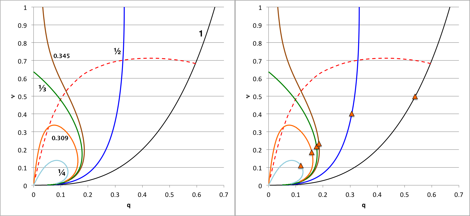
However, contrary to expectations, in no case did we find that <math>~\mathfrak{s}_\mathrm{core}/\mathfrak{s}_\mathrm{env} = 5</math>. That is to say, we found that none of the models lies on the (red-dashed) curve in the <math>~q-\nu</math> parameter space that separates stable from unstable models as defined by our above free-energy-based stability analysis. The left-hand panel of Figure 4 shows this (red-dashed) demarcation curve; for all intents and purposes, it is a reproduction of the right-hand panel of Figure 3, above — turning-point markers have been removed to minimize clutter, the equilibrium sequences have been labeled, and the horizontal axis has been extended to unity in order to include a longer portion of the <math>~\mu_e/\mu_c = 1</math> sequence. The orange triangular markers that appear in the right-hand panel of Figure 4 pinpoint where each of the Table 2 "marginally unstable" models resides in this <math>~q-\nu</math> plane. Clearly, all six of the orange triangles lie well off of — and to the stable side of — the red-dashed demarcation curve. This discrepancy, which has resulted from our use of two separate approaches to stability analysis, will be discussed further and gratifyingly resolved, below.
| Figure 4 | |||||||||
|---|---|---|---|---|---|---|---|---|---|
 |
|||||||||
Eigenfunction Details
Here we examine some of the properties of the fundamental-mode eigenfunctions that we have found are associated with marginally unstable, <math>~(n_c, n_e) = (5,1)</math> bipolytropes.
| Figure 5 |
|---|
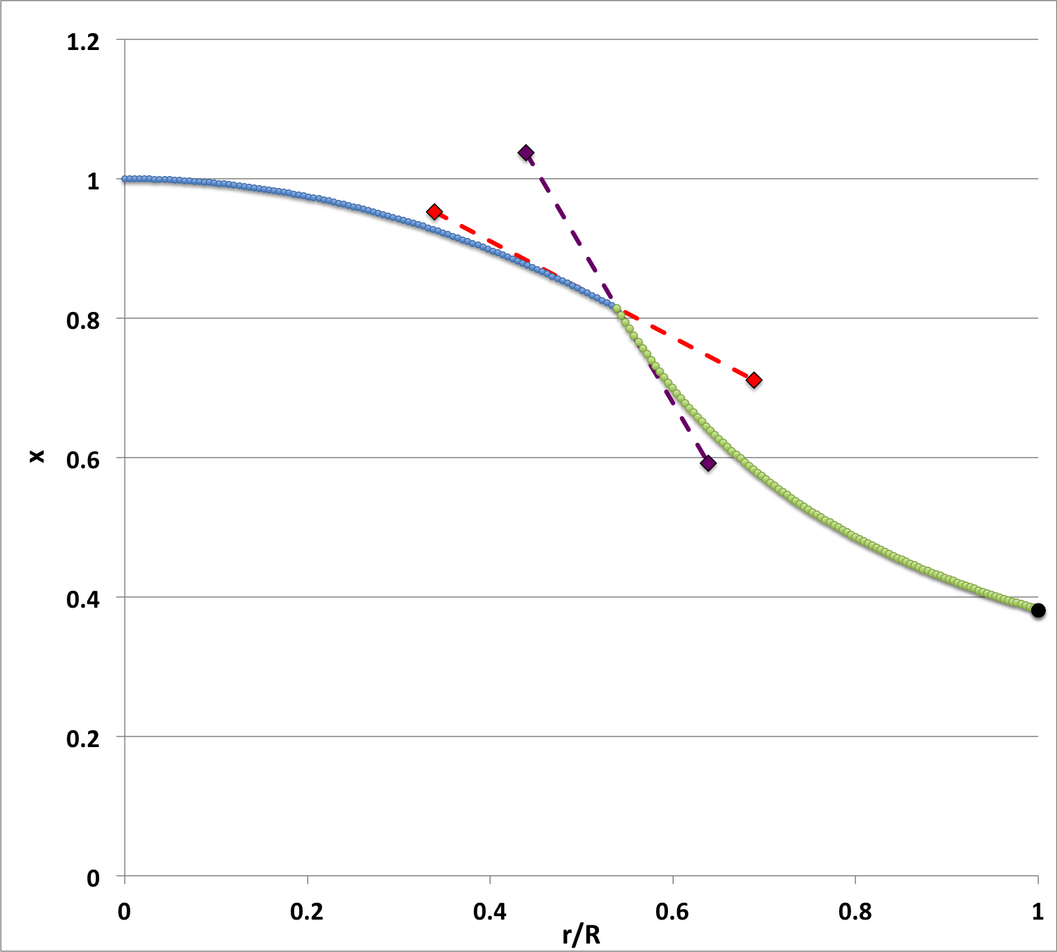
Consider the model on the <math>~\mu_e/\mu_c = 1</math> sequence for which <math>~\sigma_c^2=0~</math>: Figure 5 shows how our numerically derived, fundamental-mode eigenfunction, <math>~x = \delta r/r_0</math>, varies with the fractional radius over the entire range, <math>~0 \le r/R \le 1</math>. By prescription, the eigenfunction has a value of unity and a slope of zero at the center <math>~(r/R = 0)</math>. Integrating the LAWE outward from the center, through the model's core (blue curve segment), <math>~x</math> drops smoothly to the value <math>~x_i = 0.81437</math> at the interface <math>~(\xi_i = 1.6686460157 ~\Rightarrow~ q = r_\mathrm{core}/R_\mathrm{surf} = 0.53885819)</math>. Our numerical integration of the LAWE showed that, at the interface, the logarithmic slope of the core (blue) segment of the eigenfunction is,
|
<math>~ \biggl\{ \frac{d\ln x}{d\ln r}\biggr|_i \biggr\}_\mathrm{core} = \biggl\{ \frac{d\ln x}{d\ln \xi}\biggr|_i \biggr\}_\mathrm{core} </math> |
<math>~=</math> |
<math>~- 0.455872 \, .</math> |
Next, following the above discussion of matching conditions at the interface, we determined that, from the perspective of the envelope, the slope of the eigenfunction at the interface must therefore be,
|
<math>~ \biggl\{ \frac{d\ln x}{d\ln r}\biggr|_i \biggr\}_\mathrm{env} = \biggl\{ \frac{d\ln x}{d\ln \eta}\biggr|_i \biggr\}_\mathrm{env} </math> |
<math>~=</math> |
<math>~3\biggl(\frac{\gamma_c}{\gamma_e} -1\biggr) + \frac{\gamma_c}{\gamma_e} \biggl\{ \frac{d\ln x}{d\ln \xi}\biggr|_i \biggr\}_\mathrm{core} = -1.47352 \, .</math> |
Adopting this "env" slope along with the amplitude, <math>~x_i = 0.81437</math>, as the appropriate interface boundary conditions, we integrated the LAWE from the interface to the surface, obtaining the green-colored segment of the eigenfunction that is shown in Figure 5. The amplitude continued to steadily decrease, reaching a value of <math>~x_s = 0.38203</math>, at the model's surface <math>~(r/R = 1)</math>. At the surface, this envelope (green) segment of the eigenfunction exhibits a logarithmic slope that matches to eight significant digits the value that is expected from astrophysical arguments for this marginally unstable <math>~(\sigma_c^2=0)</math> model, namely,
<math>~ \frac{d\ln x}{d\ln \eta}\biggr|_s = \biggl[ \biggl( \frac{\rho_c}{\bar\rho} \biggr)\frac{\cancelto{0}{\sigma_c^2}}{2\gamma_e} - \biggl(3 - \frac{4}{\gamma_e}\biggr)\biggr] = -1 \, . </math>
The discontinuous jump that occurs in the slope of the eigenfunction at the interface results from our assumption that the effective adiabatic index of material in the core <math>~(\gamma_c = 6/5)</math> is different from the effective adiabatic index of the envelope material <math>~(\gamma_e = 2)</math>. In an effort to emphasize and more clearly illustrate the behavior of this fundamental-mode eigenfunction as it crosses the core/envelope interface, we have added a pair of dashed line segments to the Figure 5 plot. The red-dashed line segment touches, and is tangent to, the blue segment of the eigenfunction at the location of the core/envelope interface; it has a slope,
|
<math>~ \frac{dx}{d(r/R)}\biggr|_i = \frac{x_i}{(r_i/R)}\biggl\{ \frac{d\ln x}{d\ln r}\biggr|_i\biggr\}_\mathrm{core} </math> |
<math>~=</math> |
<math>~- 0.455872 \biggl(\frac{ 0.81437 }{ 0.53885819 }\biggr) = - 0.68895\, .</math> |
On the other hand, the purple-dashed line segment touches, and is tangent to, the green segment of the eigenfunction at the location of the core/envelope interface; it has a slope,
|
<math>~ \frac{dx}{d(r/R)}\biggr|_i = \frac{x_i}{(r_i/R)}\biggl\{ \frac{d\ln x}{d\ln r}\biggr|_i\biggr\}_\mathrm{env} </math> |
<math>~=</math> |
<math>~- 1.47352 \biggl(\frac{ 0.81437 }{ 0.53885819 }\biggr) = - 2.22691\, .</math> |
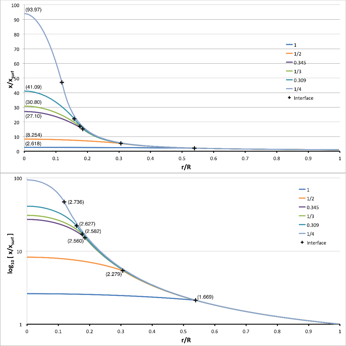
For comparison purposes, the eigenfunction shown in Figure 5 has been presented again in Figure 6, along with several other of our numerically derived eigenfunctions, but in Figure 6 its plotted amplitude has been renormalized to give a surface value of unity.
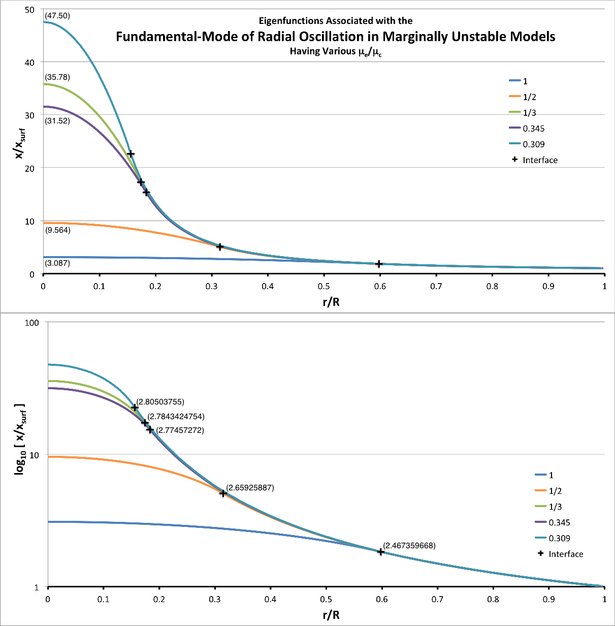
In Figure 6 we show the behavior of the fundamental-mode eigenfunction for each of the marginally unstable models identified in Table 2. In the top figure panel, each curve shows — on a linear-linear plot — how the amplitude varies with radius; in the bottom figure panel, the amplitude is plotted on a logarithmic scale. On each curve, the black plus sign marks the radial location of the core-envelope interface; in the bottom panel, these markers are accompanied by the values of <math>~\xi_i</math> that are associated with each corresponding model (see also the second column of Table 2). Each eigenfunction has been normalized such that the surface amplitude is unity. In the top panel, the value of the central amplitude of the eigenfunction that results from this normalization is recorded near the point where each eigenfunction touches the vertical axis.
|
Figure 6: Eigenfunctions Associated with the Fundamental-Mode of Radial Oscillation |
|---|
Notice that, especially as they approach the surface, the "envelope" segments of these six marginally unstable models appear to merge into the same curve, irrespective of their value of the ratio of mean molecular weights. Note as well that the "kink" that arises in the eigenfunction — due to a discontinuous jump in the slope of the eigenfunction at the core/envelope interface — becomes less and less noticeable for smaller and smaller values of the ratio of mean molecular weights.
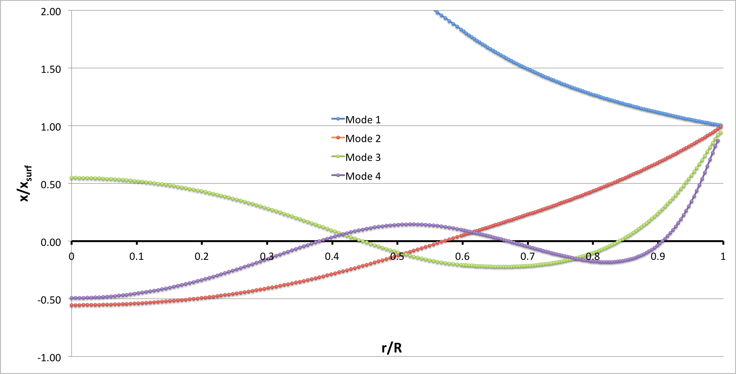
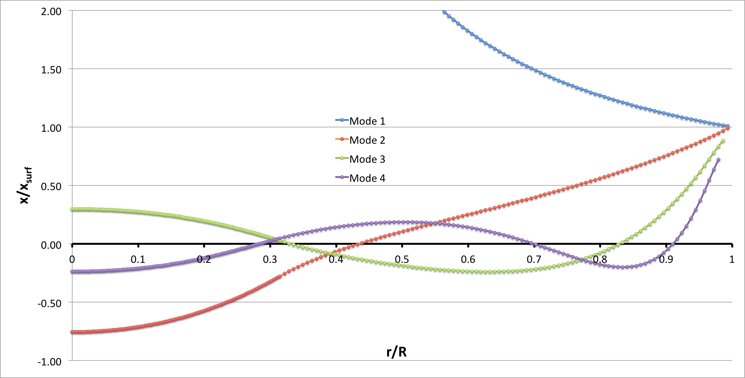
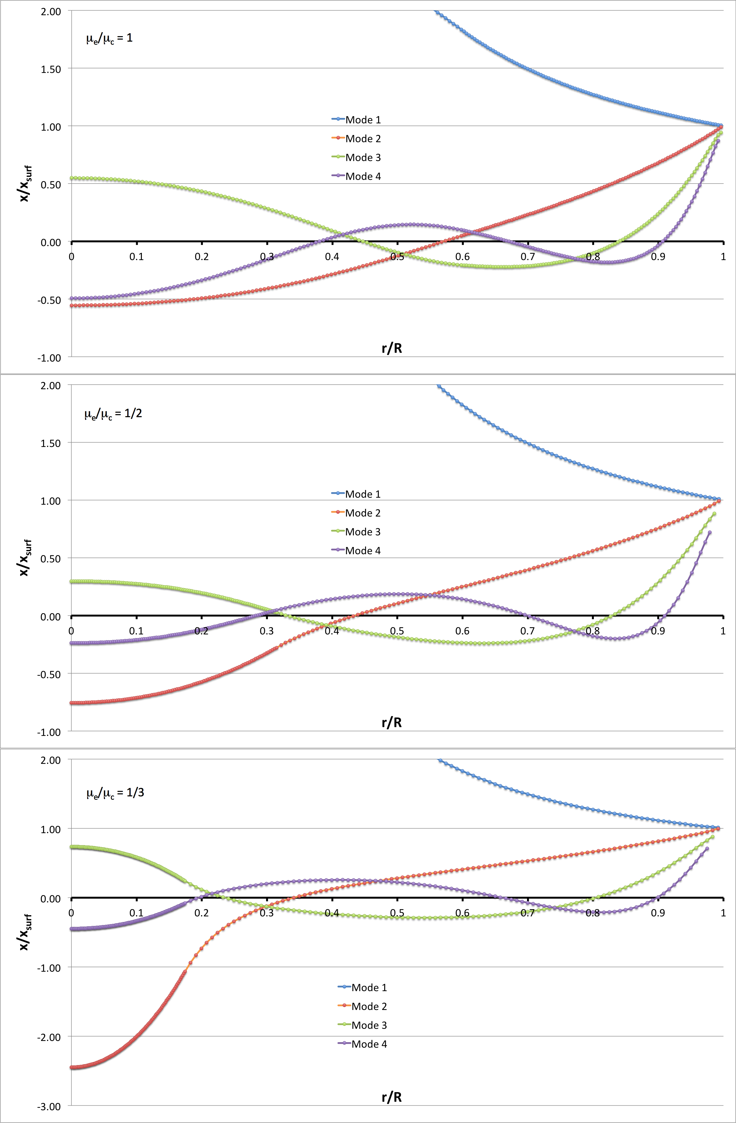
Other Modes
Summary
Reconciliation
Straight Virial Analysis
In an accompanying discussion of the viral stability of <math>~(n_c, n_e) = (5, 1)</math > bipolytropes — see also an associated discussion of the free-energy of these configurations — we find the following table of models. Let's start by finding a set of eigenvectors associated with each the subset of models highlighted in yellow.
|
|||||||||||||||||||||||||||||||||||||||||||||||||||||||||||||||||||||||||||||||||||||||||||||||||||||||||||
|
Figure 3: Largely the same as Figure 1, above, but a red-dashed curve has been added that separates the <math>~q - \nu</math> domain into regions that contain stable models (lying below the curve) from dynamically unstable models (lying above the curve), as determined by the virial stability analysis presented here. |
|||||||||||||||||||||||||||||||||||||||||||||||||||||||||||||||||||||||||||||||||||||||||||||||||||||||||||
In the context of our present discussion, we find that when <math>~\mu_e/\mu_c = 1/3</math>:
- Our virial analysis shows that the model having marginal stability has the properties: <math>~\xi = 8.548</math>, <math>~q = 0.0990</math>, and <math>~\nu = 0.4790</math>.
- In contrast, our solution to the LAWE identifies the marginally stable configuration has the properties: <math>~\xi = 2.78434248</math>, <math>~q = 0.1741</math>, and <math>~\nu = 0.2377</math>.
Variational Principle
Setup
Let's follow the guidelines of the variational principle. Instead of starting with the form of the LAWE given above, namely,
Adiabatic Wave (or Radial Pulsation) Equation
|
<math>~ \frac{d^2x}{dr_0^2} + \biggl[\frac{4}{r_0} - \biggl(\frac{g_0 \rho_0}{P_0}\biggr) \biggr] \frac{dx}{dr_0} + \biggl(\frac{\rho_0}{\gamma_\mathrm{g} P_0} \biggr)\biggl[\omega^2 + (4 - 3\gamma_\mathrm{g})\frac{g_0}{r_0} \biggr] x = 0 </math> |
we will start with a form that is more amenable to the variational principle, namely,
|
<math>~0</math> |
<math>~=</math> |
<math>~ \frac{d}{dr_0}\biggl[ r_0^4 \gamma P_0 ~\frac{dx}{dr_0} \biggr] +\biggl[ \omega^2 \rho_0 r_0^4 + (3\gamma - 4) r_0^3 \frac{dP_0}{dr_0} \biggr] x \, . </math> |
|
ASIDE: Let's show that these two expressions are equivalent. Remembering that,
the second expression becomes,
Hence, we must multiply the first expression through by <math>~r_0^4 \gamma P_0</math> in order to obtain the second expression. |
From above, we realize that multiplying the second expression through by <math>~(K_c/G)\rho_c^{-4 / 5}</math> gives,
|
<math>~0</math> |
<math>~=</math> |
<math>~ r_0^4\gamma P_0 \biggl\{ \frac{d^2x}{dr*^2} + \biggl[ 4 -\biggl(\frac{\rho^*}{P^*}\biggr)\frac{ M_r^*}{(r^*)}\biggr] \frac{1}{r^*} \frac{dx}{dr*} + \biggl(\frac{\rho^*}{ P^* } \biggr)\biggl[ \frac{2\pi \sigma_c^2}{3\gamma_\mathrm{g}} ~-~\frac{\alpha_\mathrm{g} M_r^*}{(r^*)^3}\biggr] x \biggr\} </math> |
|
|
<math>~=</math> |
<math>~ (r^*)^4 [K_c^{1 / 2}/(G^{1 / 2} \rho_c^{2/5}) ]^4 \gamma P^* [K_c\rho_c^{6/5}] \biggl\{ \frac{d^2x}{dr*^2} + \biggl[ 4 -\biggl(\frac{\rho^*}{P^*}\biggr)\frac{ M_r^*}{(r^*)}\biggr] \frac{1}{r^*} \frac{dx}{dr*} + \biggl(\frac{\rho^*}{ P^* } \biggr)\biggl[ \frac{2\pi \sigma_c^2}{3\gamma_\mathrm{g}} ~-~\frac{\alpha_\mathrm{g} M_r^*}{(r^*)^3}\biggr] x \biggr\} </math> |
|
|
<math>~=</math> |
<math>~ \biggl[ \frac{K_c^{3}}{ G^{2} \rho_c^{2/5}} \biggr] (r^*)^4 \gamma P^* \biggl\{ \frac{d^2x}{dr*^2} + \biggl[ 4 -\biggl(\frac{\rho^*}{P^*}\biggr)\frac{ M_r^*}{(r^*)}\biggr] \frac{1}{r^*} \frac{dx}{dr*} + \biggl(\frac{\rho^*}{ P^* } \biggr)\biggl[ \frac{2\pi \sigma_c^2}{3\gamma_\mathrm{g}} ~-~\frac{\alpha_\mathrm{g} M_r^*}{(r^*)^3}\biggr] x \biggr\} \, . </math> |
That is, multiplying the second expression through by, <math>~(K_c/G)\rho_c^{-4 / 5} \cdot G^2 \rho_c^{2 / 5}/K_c^3 = G/(K_c^2 \rho_c^{2 / 5})</math> , should give a desirable, totally dimensionless version of the LAWE. Remembering that,
|
<math>~\rho^*</math> |
<math>~\equiv</math> |
<math>~\frac{\rho_0}{\rho_c}</math> |
; |
<math>~r^*</math> |
<math>~\equiv</math> |
<math>~\frac{r_0}{[K_c^{1/2}/(G^{1/2}\rho_c^{2/5})]}</math> |
|
<math>~P^*</math> |
<math>~\equiv</math> |
<math>~\frac{P_0}{K_c\rho_c^{6/5}}</math> |
; |
<math>~M_r^*</math> |
<math>~\equiv</math> |
<math>~\frac{M_r}{[K_c^{3/2}/(G^{3/2}\rho_c^{1/5})]}</math> |
|
<math>~\frac{dP^*}{dr^*}</math> |
<math>~=</math> |
<math>~-\frac{M^*_r \rho^*}{(r^*)^2} </math> |
; |
<math>~E_\mathrm{norm}</math> |
<math>~=</math> |
<math>~\biggl[ \frac{K_c^5}{G^3}\biggr]^{1 / 2}</math> |
let's try it.
|
<math>~0</math> |
<math>~=</math> |
<math>~G K_c^{-2} \rho_c^{-2 / 5} \biggl\{ \frac{d}{dr_0}\biggl[ r_0^4 \gamma P_0 ~\frac{dx}{dr_0} \biggr] +\biggl[ \omega^2 \rho_0 r_0^4 + (3\gamma - 4) r_0^3 \frac{dP_0}{dr_0} \biggr] x \biggr\} </math> |
|
|
<math>~=</math> |
<math>~G K_c^{-2} \rho_c^{-2 / 5} \biggl\{ \biggl( \frac{K_c^2 \rho_c^{2/5}}{G} \biggr) \frac{d}{dr^*}\biggl[ (r^*)^4 \gamma P^* ~\frac{dx}{dr^*} \biggr] +\biggl[ \omega^2 \biggl(\frac{K_c^2}{G^2 \rho_c^{8/5}}\biggr) \rho_c \rho^* (r^*)^4 + (3\gamma - 4)\biggl(\frac{K_c }{G \rho_c^{4/5}}\biggr)K_c\rho_c^{6/5} (r^*)^3 \frac{dP^*}{dr^*} \biggr] x \biggr\} </math> |
|
|
<math>~=</math> |
<math>~ \frac{d}{dr^*}\biggl[ (r^*)^4 \gamma P^* ~\frac{dx}{dr^*} \biggr] +\biggl[ \biggl( \frac{\omega^2}{G\rho_c}\biggr) \rho^* (r^*)^4 + (3\gamma - 4)(r^*)^3 \frac{dP^*}{dr^*} \biggr] x \, . </math> |
Now, guided by the accompanying summary, if we multiply through by <math>~4\pi x dr^*</math> and integrate over the entire volume, we obtain the governing variational relation, namely,
|
<math>~0</math> |
<math>~=</math> |
<math>~\int_0^{r^*_\mathrm{core}}4\pi x\cdot d\biggl[ (r^*)^4 \gamma_c P^* ~\frac{dx}{dr^*} \biggr] + \int_0^{r^*_\mathrm{core}}\biggl[ \biggl( \frac{\omega^2}{G\rho_c}\biggr) \rho^* (r^*)^4 + (3\gamma_c - 4)(r^*)^3 \frac{dP^*}{dr^*} \biggr] 4\pi x^2 dr^* </math> |
|
|
|
<math>~ +\int_{r^*_\mathrm{core}}^{R^*}4\pi x\cdot d\biggl[ (r^*)^4 \gamma_e P^* ~\frac{dx}{dr^*} \biggr] + \int_{r^*_\mathrm{core}}^{R^*}\biggl[ \biggl( \frac{\omega^2}{G\rho_c}\biggr) \rho^* (r^*)^4 + (3\gamma_e - 4)(r^*)^3 \frac{dP^*}{dr^*} \biggr] 4\pi x^2 dr^* </math> |
|
|
<math>~=</math> |
<math>~ \biggl[ 4\pi x(r^*)^4 \gamma_c P^* ~\frac{dx}{dr^*} \biggr]_0^{r^*_\mathrm{core}} - \int_0^{r^*_\mathrm{core}}4\pi \biggl[ (r^*)^4 \gamma_c P^* ~\biggl( \frac{dx}{dr^*} \biggr)^2\biggr] dr^* - \int_0^{r^*_\mathrm{core}}\biggl[ (3\gamma_c - 4)M^*_r \rho^* \biggr] 4\pi x^2 r^* dr^* </math> |
|
|
|
<math>~ +\biggl[ 4\pi x(r^*)^4 \gamma_e P^* ~\frac{dx}{dr^*} \biggr]_{r^*_\mathrm{core}}^{R^*} - \int_{r^*_\mathrm{core}}^{R^*}4\pi \biggl[ (r^*)^4 \gamma_e P^* ~\biggl( \frac{dx}{dr^*} \biggr)^2\biggr] dr^* - \int_{r^*_\mathrm{core}}^{R^*}\biggl[ (3\gamma_e - 4)M^*_r \rho^* \biggr] 4\pi x^2 r^* dr^* + \int_{0}^{R^*}\biggl[ \biggl( \frac{\omega^2}{G\rho_c}\biggr) \rho^* (r^*)^4 \biggr] 4\pi x^2 dr^* </math> |
|
|
<math>~=</math> |
<math>~ - \int_0^{r^*_\mathrm{core}} x^2~\biggl( \frac{d\ln x}{d\ln r^*} \biggr)^2 \gamma_c 4\pi (r^*)^2 P^* dr^* + \int_0^{r^*_\mathrm{core}} (3\gamma_c - 4) x^2\biggl( -\frac{M^*_r}{r^*}\biggr) 4\pi \rho^* (r^*)^2 dr^* -\biggl[ 4\pi x^2 (r^*)^3 \gamma_c P^* \biggl( - \frac{d\ln x}{d\ln r^*} \biggr) \biggr]_0^{r^*_\mathrm{core}} </math> |
|
|
|
<math>~ - \int_{r^*_\mathrm{core}}^{R^*} x^2~\biggl( \frac{d\ln x}{d\ln r^*} \biggr)^2 \gamma_e 4\pi (r^*)^2 P^* dr^* + \int_{r^*_\mathrm{core}}^{R^*} (3\gamma_e - 4) x^2\biggl( -\frac{M^*_r}{r^*}\biggr) 4\pi \rho^* (r^*)^2 dr^* -\biggl[ 4\pi x^2 (r^*)^3 \gamma_e P^* \biggl( - \frac{d\ln x}{d\ln r^*} \biggr) \biggr]_{r^*_\mathrm{core}}^{R^*} + \int_{0}^{R^*} 4\pi \biggl( \frac{\omega^2}{G\rho_c}\biggr) \rho^* (r^*)^4 x^2 dr^* \, . </math> |
Energy Normalization:
|
<math>~(\gamma - 1)dU_\mathrm{int}</math> |
<math>~=</math> |
<math>~ 4\pi r^2 P dr </math> |
|
|
<math>~=</math> |
<math>~ 4\pi \biggl[ \frac{K_c^{1 / 2}}{G^{1 / 2} \rho_c^{2 / 5}} \biggr]^3 K_c \rho_c^{6 / 5} (r^*)^2 P^* dr^* </math> |
|
|
<math>~=</math> |
<math>~ 4\pi \biggl[ \frac{K_c^{5}}{G^{3}} \biggr]^{1 / 2} (r^*)^2 P^* dr^* </math> |
|
<math>~\Rightarrow ~~~ E_\mathrm{norm}</math> |
<math>~\equiv</math> |
<math>~ \biggl[ \frac{K_c^{5}}{G^{3}} \biggr]^{1 / 2} </math> |
|
<math>~dW_\mathrm{grav}</math> |
<math>~=</math> |
<math>~ -\biggl( \frac{GM_r}{r} \biggr) 4\pi r^2 \rho dr </math> |
|
|
<math>~=</math> |
<math>~ -\biggl( \frac{GM^*_r}{r^*} \biggr) 4\pi (r^*)^2 \rho^* dr^* \biggl[ \frac{K_c}{G\rho_c^{4 / 5}} \biggr]\rho_c \biggl[ \frac{ K_c^{3 / 2} }{G^{3 / 2}\rho_c^{1 / 5} } \biggr] </math> |
|
|
<math>~=</math> |
<math>~ -\biggl( \frac{M^*_r}{r^*} \biggr) 4\pi (r^*)^2 \rho^* dr^* E_\mathrm{norm} </math> |
Hence, the dimensionless governing variational relation becomes,
|
<math>~\int_0^{R^*} \biggl( \frac{2\pi}{3}\biggr)\sigma_c^2(r^*)^2 x^2 dM_r^* </math> |
<math>~=</math> |
<math>~ \int_0^{r^*_\mathrm{core}} \gamma_c(\gamma_c - 1) x^2~\biggl( \frac{d\ln x}{d\ln r^*} \biggr)^2 dU^*_\mathrm{int}
- \int_0^{r^*_\mathrm{core}} (3\gamma_c - 4) x^2 dW^*_\mathrm{grav} + \biggl[ 4\pi x^2 (r^*)^3 \gamma_c P^* \biggl( - \frac{d\ln x}{d\ln r^*} \biggr) \biggr]_0^{r^*_\mathrm{core}} </math> |
|
|
|
<math>~ + \int_{r^*_\mathrm{core}}^{R^*} \gamma_e(\gamma_e - 1) x^2~\biggl( \frac{d\ln x}{d\ln r^*} \biggr)^2 dU^*_\mathrm{int} - \int_{r^*_\mathrm{core}}^{R^*} (3\gamma_e - 4) x^2 dW^*_\mathrm{grav} + \biggl[ 4\pi x^2 (r^*)^3 \gamma_e P^* \biggl( - \frac{d\ln x}{d\ln r^*} \biggr) \biggr]_{r^*_\mathrm{core}}^{R^*} </math> |
|
|
<math>~=</math> |
<math>~ \frac{2\gamma_c}{3} \int_0^{r^*_\mathrm{core}} x^2~\biggl( \frac{d\ln x}{d\ln r^*} \biggr)^2 dS^*_\mathrm{therm} - (3\gamma_c - 4) \int_0^{r^*_\mathrm{core}} x^2 dW^*_\mathrm{grav} + 4\pi x_i^2 (r_\mathrm{core}^*)^3 \gamma_c P_i^* \biggl\{ - \frac{d\ln x}{d\ln r^*}\biggr|_i \biggr\}_\mathrm{core} </math> |
|
|
|
<math>~ + \frac{2 \gamma_e}{3}\int_{r^*_\mathrm{core}}^{R^*} x^2~\biggl( \frac{d\ln x}{d\ln r^*} \biggr)^2 dS^*_\mathrm{therm} - (3\gamma_e - 4) \int_{r^*_\mathrm{core}}^{R^*} x^2 dW^*_\mathrm{grav} - 4\pi x_i^2 (r_\mathrm{core}^*)^3 \gamma_e P_i^* \biggl\{ - \frac{d\ln x}{d\ln r^*}\biggr|_i \biggr\}_\mathrm{env} </math> |
|
|
<math>~=</math> |
<math>~ \frac{2\gamma_c}{3} \int_0^{r^*_\mathrm{core}} x^2~\biggl( \frac{d\ln x}{d\ln r^*} \biggr)^2 dS^*_\mathrm{therm} - (3\gamma_c - 4) \int_0^{r^*_\mathrm{core}} x^2 dW^*_\mathrm{grav} </math> |
|
|
|
<math>~ + \frac{2 \gamma_e}{3}\int_{r^*_\mathrm{core}}^{R^*} x^2~\biggl( \frac{d\ln x}{d\ln r^*} \biggr)^2 dS^*_\mathrm{therm} - (3\gamma_e - 4) \int_{r^*_\mathrm{core}}^{R^*} x^2 dW^*_\mathrm{grav} + 4\pi x_i^2 (r_\mathrm{core}^*)^3 P_i^*\biggl[ \gamma_c \biggl\{ - \frac{d\ln x}{d\ln r^*}\biggr|_i \biggr\}_\mathrm{core} - \gamma_e \biggl\{ - \frac{d\ln x}{d\ln r^*}\biggr|_i \biggr\}_\mathrm{env} \biggr] </math> |
|
|
<math>~=</math> |
<math>~ \frac{2\gamma_c}{3} \int_0^{r^*_\mathrm{core}} x^2~\biggl( \frac{d\ln x}{d\ln r^*} \biggr)^2 dS^*_\mathrm{therm} - (3\gamma_c - 4) \int_0^{r^*_\mathrm{core}} x^2 dW^*_\mathrm{grav} </math> |
|
|
|
<math>~ + \frac{2 \gamma_e}{3}\int_{r^*_\mathrm{core}}^{R^*} x^2~\biggl( \frac{d\ln x}{d\ln r^*} \biggr)^2 dS^*_\mathrm{therm} - (3\gamma_e - 4) \int_{r^*_\mathrm{core}}^{R^*} x^2 dW^*_\mathrm{grav} + 4\pi x_i^2 (r_\mathrm{core}^*)^3 P_i^*\biggl[ 3(\gamma_e - \gamma_c) \biggr] \, , </math> |
where,
|
<math>~dM^*_r</math> |
<math>~=</math> |
<math>~4\pi (r^*)^2 \rho^* dr^* \, ,</math> |
|
<math>~dU^*_\mathrm{int}</math> |
<math>~=</math> |
<math>~\frac{1}{(\gamma-1)} \biggl[4\pi (r^*)^2 P^* dr^* \biggr] = \biggl[ \frac{2}{3(\gamma - 1)} \biggr]dS^*_\mathrm{therm} \, ,</math> |
|
<math>~dW^*_\mathrm{grav}</math> |
<math>~=</math> |
<math>~-\biggl( \frac{M^*_r}{r^*} \biggr) 4\pi (r^*)^2 \rho^* dr^* \, .</math> |
Implementation
|
Table 3 |
|||||||||||||||||||||||||||||||||||||||||
|---|---|---|---|---|---|---|---|---|---|---|---|---|---|---|---|---|---|---|---|---|---|---|---|---|---|---|---|---|---|---|---|---|---|---|---|---|---|---|---|---|---|
| <math>~\frac{\mu_e}{\mu_c}</math> | <math>~\xi_i</math> | Core | Envelope | ||||||||||||||||||||||||||||||||||||||
| Integrals over<math>~dS^*_\mathrm{therm}</math> | Integrals over<math>~dW^*_\mathrm{grav}</math> | Integrals over<math>~dS^*_\mathrm{therm}</math> | Integrals over<math>~dW^*_\mathrm{grav}</math> | ||||||||||||||||||||||||||||||||||||||
| Analytic <math>~\mathfrak{s}_\mathrm{core}</math> |
Numerical <math>~\mathfrak{s}_\mathrm{core}</math> |
TERM1 | Analytic <math>~\mathfrak{w}_\mathrm{core}</math> |
Numerical <math>~\mathfrak{w}_\mathrm{core}</math> |
TERM2 | Analytic <math>~\mathfrak{s}_\mathrm{core}</math> |
Numerical <math>~\mathfrak{s}_\mathrm{core}</math> |
TERM3 | Analytic <math>~\mathfrak{w}_\mathrm{core}</math> |
Numerical <math>~\mathfrak{w}_\mathrm{core}</math> |
TERM4 | ||||||||||||||||||||||||||||||
| 1 | 1.6686460157 | 3.021916335 | 3.021921 | 0.116389175 | -3.356583022 | -3.35666 | -2.649752079 | 1.47780476 | 1.47791 | 1.0720821 | -5.642859167 | -5.642820 | -1.91142893 | ||||||||||||||||||||||||||||
| <math>~\tfrac{1}{2}</math> | 2.27925811317 | 4.241287117 | 4.241410819 | 0.352702823 | -6.074241035 | -6.074317546 | +1.66029247 | 4.284931508 | 4.28547195 | 1.92869243 | -10.97819621 | -10.97847622 | -1.85197268 | ||||||||||||||||||||||||||||
| 0.345 | 2.560146865247 | 4.639705843 | -7.125754184 | 11.72861751 | -25.61089252 | ||||||||||||||||||||||||||||||||||||
| <math>~\tfrac{1}{3}</math> | 2.582007485476 | 4.667042505 | -7.200966267 | 13.15887139 | -28.45086152 | ||||||||||||||||||||||||||||||||||||
| 0.309 | 2.6274239687695 | 4.722277318 | -7.354156963 | 17.1374434 | -36.36528446 | ||||||||||||||||||||||||||||||||||||
| <math>~\tfrac{1}{4}</math> | 2.7357711469398 | 4.84592201 | -7.70305421 | 37.84289623 | -77.67458196 | ||||||||||||||||||||||||||||||||||||
|
|||||||||||||||||||||||||||||||||||||||||
|
<math>~ \sigma_c^2</math> |
<math>~=</math> |
<math>~\frac{3}{2\pi \cdot \mathbf{TERM5} } \biggl\{ \frac{2\gamma_c}{3} [\mathbf{TERM1}] - (3\gamma_c - 4) [\mathbf{TERM2}] + \frac{2 \gamma_e}{3} [\mathbf{TERM3}] - (3\gamma_e - 4) [\mathbf{TERM4}] </math> |
|
|
|
<math>~ + 4\pi x_i^2 (r_\mathrm{core}^*)^3 P_i^* \biggl[ \gamma_c \biggl\{ - \frac{d\ln x}{d\ln r^*}\biggr|_i \biggr\}_\mathrm{core} - \gamma_e \biggl\{ - \frac{d\ln x}{d\ln r^*}\biggr|_i \biggr\}_\mathrm{env}\biggr] \biggr\} </math> |
<math>~\sigma_c^2 = 0.036312577\times \biggl[0.093111340 - 1.059900832 + 1.4294428 - (-3.82285786) + 1.782200484\times (-2.399993628) \biggr] = 0.036312577\times [0.00819] = 0.0002973 \, .</math>
|
Table 4 |
|||||||||||||||||
|---|---|---|---|---|---|---|---|---|---|---|---|---|---|---|---|---|---|
| <math>~\frac{\mu_e}{\mu_c}</math> | <math>~\xi_i</math> | Analytic <math>~\mathfrak{m}_\mathrm{tot}</math> |
Numerical <math>~\mathfrak{m}_\mathrm{tot}</math> |
TERM5 | <math>~x_i</math> | <math>~r^*_\mathrm{core}</math> | <math>~P^*_i</math> | <math>~\biggl\{ - \frac{d\ln x}{d\ln r^*}\biggr|_i \biggr\}_\mathrm{core}</math> | <math>~\biggl\{ - \frac{d\ln x}{d\ln r^*}\biggr|_i \biggr\}_\mathrm{env}</math> | <math>~\sigma_c^2</math> | |||||||
| 1 | 1.6686460157 | 4.818155928 | 4.818145 | 13.14874521 | 0.814374698 | 1.153014872 | 0.139506172 | +0.455871977 | +1.47352 | 0.000297 | |||||||
| <math>~\tfrac{1}{2}</math> | 2.27925811317 | ||||||||||||||||
| 0.345 | 2.560146865247 | ||||||||||||||||
| <math>~\tfrac{1}{3}</math> | 2.582007485476 | ||||||||||||||||
| 0.309 | 2.6274239687695 | ||||||||||||||||
| <math>~\tfrac{1}{4}</math> | 2.7357711469398 | ||||||||||||||||
|
|||||||||||||||||
See Also
- K. De et al. (12 October 2018, Science, Vol. 362, No. 6411, pp. 201 - 206), A Hot and Fast Ultra-stripped Supernova that likely formed a Compact Neutron Star Binary.

|
|---|
|
© 2014 - 2021 by Joel E. Tohline |
