User:Tohline/SSC/Structure/BiPolytropes/Analytic1 5
BiPolytrope with <math>n_c = 1</math> and <math>n_e=5</math>

|
|---|
| | Tiled Menu | Tables of Content | Banner Video | Tohline Home Page | |
Here we construct a system of bipolytropic configurations in which the core has an <math>~n_c=1</math> polytropic index and the envelope has an <math>~n_e=5</math> polytropic index. As in the case of our separately discussed, "mirror image" bipolytropic configurations having <math>~(n_c, n_e) = (5, 1)</math>, this system is particularly interesting because the entire structure can be described by closed-form, analytic expressions. Bipolytropes of this type were first constructed by J. O. Murphy (1983, Proc. Astr. Soc. of Australia, 5, 175), and attributes of their physical structure were further discussed by J. O. Murphy & R. Fiedler (1985a, Proc. Astr. Soc. of Australia, 6, 219); additional, closely related references are given below. In the discussion that follows, we will be heavily referencing Murphy's (1983) work.
Steps 2 & 3
Based on the discussion presented elsewhere of the structure of an isolated <math>~n=1</math> polytrope, the core of this bipolytrope will have the following properties:
<math> \theta(\xi) = \frac{\sin\xi}{\xi} ~~~~\Rightarrow ~~~~ \theta_i = \frac{\sin\xi_i}{\xi_i} ; </math>
<math> \frac{d\theta}{d\xi} = \biggl[ \frac{\cos\xi}{\xi}- \frac{\sin\xi}{\xi^2}\biggr] ~~~~\Rightarrow ~~~~ \biggl(\frac{d\theta}{d\xi}\biggr)_i = \biggl[\frac{\cos\xi_i}{\xi_i}- \frac{\sin\xi_i}{\xi_i^2} \biggr] \, . </math>
The first zero of the function <math>~\theta(\xi)</math> and, hence, the surface of the corresponding isolated <math>~n=1</math> polytrope is located at <math>~\xi_s = \pi</math>. Hence, the interface between the core and the envelope can be positioned anywhere within the range, <math>~0 < \xi_i < \pi</math>.
Step 4: Throughout the core (<math>0 \le \xi \le \xi_i</math>)
|
Specify: <math>~K_c</math> and <math>~\rho_0 ~\Rightarrow</math> |
|
|||
|
<math>~\rho</math> |
<math>~=</math> |
<math>\rho_0 \theta^{n_c}</math> |
<math>~=</math> |
<math>~\rho_0 \biggl( \frac{\sin\xi}{\xi} \biggr)</math> |
|
<math>~P</math> |
<math>~=</math> |
<math>~K_c \rho_0^{1+1/n_c} \theta^{n_c + 1}</math> |
<math>~=</math> |
<math>~K_c \rho_0^{2} \biggl( \frac{\sin\xi}{\xi}\biggr)^{2}</math> |
|
<math>~r</math> |
<math>~=</math> |
<math>~\biggl[ \frac{(n_c + 1)K_c}{4\pi G} \biggr]^{1/2} \rho_0^{(1-n_c)/(2n_c)} \xi</math> |
<math>~=</math> |
<math>~\biggl[ \frac{K_c}{2\pi G} \biggr]^{1/2} \xi</math> |
|
<math>~M_r</math> |
<math>~=</math> |
<math>~4\pi \biggl[ \frac{(n_c + 1)K_c}{4\pi G} \biggr]^{3/2} \rho_0^{(3-n_c)/(2n_c)} \biggl(-\xi^2 \frac{d\theta}{d\xi} \biggr)</math> |
<math>~=</math> |
<math>~4\pi \biggl[ \frac{K_c}{2\pi G} \biggr]^{3/2} \rho_0 \biggl[\sin\xi - \xi \cos\xi \biggr]</math> |
Step 5: Interface Conditions
|
|
Setting <math>~n_c=1</math> and <math>~n_e=5~~~~~\Rightarrow</math> |
|||
|
<math>~\frac{\rho_e}{\rho_0}</math> |
<math>~=</math> |
<math>~\biggl( \frac{\mu_e}{\mu_c} \biggr) \theta^{n_c}_i \phi_i^{-n_e}</math> |
<math>~=</math> |
<math>~\biggl( \frac{\mu_e}{\mu_c} \biggr) \theta_i \phi_i^{-5}</math> |
|
<math>~\biggl( \frac{K_e}{K_c} \biggr) </math> |
<math>~=</math> |
<math>~\rho_0^{1/n_c - 1/n_e}\biggl( \frac{\mu_e}{\mu_c} \biggr)^{-(1+1/n_e)} \theta^{1 - n_c/n_e}_i</math> |
<math>~=</math> |
<math>~\biggl[\rho_0^{4}\biggl( \frac{\mu_e}{\mu_c} \biggr)^{-6} \theta^{4}_i\biggr]^{1/5}</math> |
|
<math>~\frac{\eta_i}{\xi_i}</math> |
<math>~=</math> |
<math>~\biggl[ \frac{n_c + 1}{n_e+1} \biggr]^{1/2} \biggl( \frac{\mu_e}{\mu_c}\biggr) \theta_i^{(n_c-1)/2} \phi_i^{(1-n_e)/2}</math> |
<math>~=</math> |
<math>~\biggl( \frac{1}{3} \biggr)^{1/2} \biggl( \frac{\mu_e}{\mu_c}\biggr) \phi_i^{-2}</math> |
|
<math>~\biggl( \frac{d\phi}{d\eta} \biggr)_i</math> |
<math>~=</math> |
<math>~\biggl[ \frac{n_c + 1}{n_e + 1} \biggr]^{1/2} \theta_i^{- (n_c + 1)/2} \phi_i^{(n_e+1)/2} \biggl( \frac{d\theta}{d\xi} \biggr)_i</math> |
<math>~=</math> |
<math>~\biggl( \frac{1}{3} \biggr)^{1/2} \theta_i^{- 1} \biggl( \frac{d\theta}{d\xi} \biggr)_i \phi_i^3</math> |
Alternative: In our introductory description of how to build a bipolytropic structure, we pointed out that, instead of employing these last two fitting conditions, Chandrasekhar [C67] found it useful to employ, instead, the ratio of the <math>3^\mathrm{rd}</math> to <math>4^\mathrm{th}</math> expressions, which in the present case produces,
<math> \frac{\eta_i \phi_i^{5}}{(d\phi/d\eta)_i} = \frac{\xi_i \theta_i}{(d\theta/d\xi)_i} \biggl( \frac{\mu_e}{\mu_c}\biggr) \, , </math>
and the product of the <math>3^\mathrm{rd}</math> and <math>4^\mathrm{th}</math> expressions, which in the present case generates,
<math> \frac{3\eta_i (d\phi/d\eta)_i}{ \phi_i } = \frac{\xi_i (d\theta/d\xi)_i}{ \theta_i } \biggl( \frac{\mu_e}{\mu_c}\biggr) \, . </math>
In what follows we will sometimes refer to the first of these two expressions as Chandrasekhar's "U-constraint" and we will sometimes refer to the second as Chandrasekhar's "V-constraint." As is explained in an accompanying discussion, Murphy (1983) followed Chandrasekhar's lead and extracted fitting conditions from this last pair of expressions. In seeking the most compact analytic solution, we have found it advantageous to invoke our standard <math>3^\mathrm{rd}</math> fitting expression in tandem with the Chandrasekhar's V-constraint.
Step 6: Envelope Solution
Following the work of Murphy (1983) and of Murphy & Fiedler (1985a), we will adopt for the envelope's structure the F-Type solution of the <math>~n=5</math> Lane-Emden function discovered by S. Srivastava (1968, ApJ, 136, 680) and described in an accompanying discussion, namely,
|
<math>~\phi</math> |
<math>~=</math> |
<math>~\frac{B_0^{-1}\sin[\ln(A_0\eta)^{1/2})]}{\eta^{1/2}\{3-2\sin^2[\ln(A_0\eta)^{1/2}]\}^{1/2}} </math> |
|
|
<math>~=</math> |
<math>~\frac{B_0^{-1}\sin\Delta}{\eta^{1/2}(3-2\sin^2\Delta)^{1/2}} \, ,</math> |
where <math>~A_0</math> is a "homology factor" and <math>~B_0</math> is an overall scaling coefficient — the values of both will be determined presently from the interface conditions — and we have introduced the notation,
<math>~\Delta \equiv \ln(A_0\eta)^{1/2} = \frac{1}{2} (\ln A_0 + \ln\eta) \, .</math>
The first derivative of Srivastava's function is,
|
<math>~\frac{d\phi}{d\eta}</math> |
<math>~=</math> |
<math>~ \frac{B_0^{-1}[3\cos\Delta-3\sin\Delta + 2\sin^3\Delta] }{2\eta^{3/2}(3-2\sin^2\Delta)^{3/2}} \, . </math> |
As has been explained in the context of our more general discussion of Srivastava's function, if we ignore, for the moment, the additional "<math>m\pi</math>" phase shift that can be attached to a determination of the angle, <math>~\Delta</math>, the physically viable interval for the dimensionless radial coordinate is, <math>~e^{2\pi} \ge A_0\eta \ge \eta_\mathrm{crit} \equiv e^{2\tan^{-1}(1+2^{1/3})} \, .</math>
For this bipolytropic configuration, it is worth emphasizing how the dimensionless radial coordinate of the <math>~n_e = 5</math> envelope, <math>~\eta</math>, is related to the dimensionless radial coordinate of the <math>~n_c = 1</math> core, <math>~\xi</math>. Referring to the general setup procedure for constructing any bipolytropic configuration that has been presented in tabular form in a separate discussion, it is clear that in order for the radial coordinate, <math>~r</math>, to carry a consistent meaning throughout the model, we must have,
|
<math>~r = \biggl[ \frac{(n_c + 1)K_c}{4\pi G} \biggr]^{1/2} \rho_0^{(1-n_c)/(2n_c)} \xi</math> |
<math>~=</math> |
<math>~\biggl[ \frac{(n_e + 1)K_e}{4\pi G} \biggr]^{1/2} \rho_e^{(1-n_e)/(2n_e)} \eta</math> |
|
<math>~\Rightarrow ~~~~\biggl( \frac{K_c}{3K_e} \biggr)\rho_e^{4/5} </math> |
<math>~=</math> |
<math>~\biggl(\frac{\eta}{\xi}\biggr)^2 \, .</math> |
Referring back to the already established interface conditions, above, to relate <math>~\rho_e</math> to <math>~\rho_0</math>, and to re-express the ratio, <math>~K_e/K_c</math>, we therefore have,
|
<math>~\biggl(\frac{\eta}{\xi}\biggr)^2</math> |
<math>~=</math> |
<math>~\frac{1}{3} \biggl[ \rho_0^{4}\biggl( \frac{\mu_e}{\mu_c} \biggr)^{-6} \theta^{4}_i\biggr]^{-1/5} \biggl[ \rho_0\biggl( \frac{\mu_e}{\mu_c} \biggr) \theta_i \phi_i^{-5} \biggr]^{4/5} </math> |
|
<math>~\Rightarrow ~~~~ \frac{\eta}{\xi}</math> |
<math>~=</math> |
<math>~\biggl(\frac{1}{3}\biggr)^{1/2} \biggl( \frac{\mu_e}{\mu_c} \biggr) \phi_i^{-2} \, .</math> |
While this result is not a surprise because the right-hand-side is the same expression that was presented, above, as the interface condition for the ratio, <math>~\eta_i/\xi_i</math>, it is nevertheless useful because it shows that the same relation works throughout the system — not just at the interface — and it clearly defines how we can swap back and forth between the two dimensionless radial coordinates when examining the structure and characteristics of this composite bipolytropic structure.
First Constraint
Calling upon Chandrasekhar's V-constraint, as just defined above — see also our accompanying discussion for elaboration on Murphy's (1983) "V5F" and "V1E" function notations — one fitting condition at the interface is,
|
<math>~- \frac{2\xi_i }{ 3\theta_i } \biggl( \frac{d\theta}{d\xi} \biggr)_i \biggl( \frac{\mu_e}{\mu_c}\biggr)</math> |
<math>~=</math> |
<math>~2\biggl[ \frac{\eta (- d\phi/d\eta)}{\phi} \biggr]_i </math> |
|
|
<math>~=</math> |
<math>~\frac{[3\sin\Delta_i - 2\sin^3\Delta_i -3\cos\Delta_i ] }{\sin\Delta_i (3-2\sin^2\Delta_i)}</math> |
|
|
<math>~=</math> |
<math>~\frac{3 - 2\sin^2\Delta_i -3\cot\Delta_i}{(3-2\sin^2\Delta_i)} \, .</math> |
The left-hand side of this expression is inherently positive over the physically viable radial coordinate range, <math>~0 \ge \xi_i \ge \pi</math> and its value is known once the radial coordinate of the edge of the core has been specified. So, defining the interface parameter,
<math>~ \kappa_i \equiv - \frac{2\theta_i^' \xi_i}{3\theta_i} \biggl( \frac{\mu_e}{\mu_c} \biggr) \, ,</math>
we will recast the first constraint into, what will henceforth be referred to as, the
|
Key Nonlinear Interface Relation
|
In a separate subsection of this chapter, below, we present a closed-form analytic solution, <math>~\Delta_i(\kappa_i)</math>, to this nonlinear equation.
Second Constraint
Obtained from Third Interface Condition
Our 3rd interface condition, as detailed above, states that,
|
<math>~\frac{\eta_i}{\xi_i}</math> |
<math>~=</math> |
<math>~3^{-1/2} \biggl( \frac{\mu_e}{\mu_c} \biggr) \phi_i^{-2} \, .</math> |
If we now choose to normalize the interface amplitude such that, <math>~\phi_i = 1</math>, then this condition establishes two relations: First, from the 3rd interface condition alone,
|
<math>~\eta_i</math> |
<math>~=</math> |
<math>~3^{-1/2} \biggl( \frac{\mu_e}{\mu_c} \biggr) \xi_i \, ;</math> |
and, second, from the definition of Srivastava's function, <math>~\phi</math>, we deduce that the overall scaling parameter is,
|
<math>~B_0^2</math> |
<math>~=</math> |
<math>~\frac{\sin^2\Delta_i}{\eta_i(3-2\sin^2\Delta_i)} </math> |
|
|
<math>~=</math> |
<math>~\frac{\sqrt{3}}{\xi_i} \biggl( \frac{\mu_e}{\mu_c} \biggr)^{-1} \biggl( \frac{3}{\sin^2\Delta_i} - 2\biggr)^{-1} \, . </math> |
Notice that, after the solution, <math>~\Delta_i(\kappa_i)</math>, of the key nonlinear interface relation has been determined, the first of these two relations also permits us to write,
|
<math>~A_0\eta_i</math> |
<math>~=</math> |
<math>~e^{2\Delta_i}</math> |
|
<math>~\Rightarrow ~~~~ A_0</math> |
<math>~=</math> |
<math>~3^{1/2} \biggl( \frac{\mu_e}{\mu_c} \biggr)^{-1} \xi_i^{-1} e^{2\Delta_i} \, .</math> |
Throughout the envelope, therefore, the angle,
|
<math>~\Delta</math> |
<math>~=</math> |
<math>~\ln(A_0\eta)^{1/2} = \frac{1}{2} \ln\biggl[ \xi \cdot \xi_i^{-1} e^{2\Delta_i} \biggr] = \Delta_i + \ln\biggl( \frac{\xi}{\xi_i} \biggr)^{1/2} \, .</math> |
Obtained from Chandrasekhar's U-constraint
We shall now demonstrate that the same expression for the scaling coefficient, <math>~B_0</math>, can alternatively be obtained from Chandrasekhar's U-constraint, without assuming that <math>~\phi_i = 1</math>, after taking into account the result that already has been obtained from the V-constraint. As described above, the U-constraint is an alternative interface condition that may be written as,
|
<math>~\frac{\xi_i \theta_i}{(-d\theta/d\xi)_i} \biggl( \frac{\mu_e}{\mu_c}\biggr)</math> |
<math>~=</math> |
<math>~\frac{\eta_i \phi_i^{5}}{(-d\phi/d\eta)_i} \, ,</math> |
which, in the particular case being examined here, becomes — again, see our accompanying discussion for elaboration on Murphy's (1983) "U5F" and "U1E" function notations —
|
<math>~\frac{2\xi_i^2}{3\kappa_i} \biggl( \frac{\mu_e}{\mu_c}\biggr)^2 </math> |
<math>~=</math> |
<math>~\biggl( U_\mathrm{5F} \biggr)_i </math> |
|
|
<math>~=</math> |
<math>~ \frac{2B_0^{-4} \sin^4\Delta_i}{(3-2\sin^2\Delta_i)(3 - 2\sin^2\Delta_i - 3\cot\Delta_i)} \, . </math> |
Now, from our discussion, above, of the first constraint, we know that,
|
<math>~(3 - 2\sin^2\Delta_i - 3\cot\Delta_i)</math> |
<math>~=</math> |
<math>~(3-2\sin^2\Delta_i)\kappa_i \, .</math> |
Hence, Chandrasekhar's U-constraint becomes,
|
<math>~\frac{2\xi_i^2}{3\kappa_i} \biggl( \frac{\mu_e}{\mu_c}\biggr)^2 </math> |
<math>~=</math> |
<math>~ \frac{2B_0^{-4} \sin^4\Delta_i}{(3-2\sin^2\Delta_i)^2 \kappa_i} </math> |
|
<math>~\Rightarrow ~~~~ B_0^4 </math> |
<math>~=</math> |
<math>~ \frac{3\sin^4\Delta_i}{\xi_i^2 (3-2\sin^2\Delta_i)^2} \biggl( \frac{\mu_e}{\mu_c}\biggr)^{-2} </math> |
|
<math>~\Rightarrow ~~~~ B_0^2</math> |
<math>~=</math> |
<math>~\frac{\sqrt{3}}{\xi_i} \biggl( \frac{\mu_e}{\mu_c} \biggr)^{-1} \biggl( \frac{3}{\sin^2\Delta_i} - 2\biggr)^{-1} \, ,</math> |
which, as predicted, is identical to what we learned from the third interface condition, alone.
Comment on Murphy's Scalings
Murphy's (1983) derivations also include an homology factor, <math>~A</math>, and an overall scaling factor, <math>~B</math>, but they are calculated differently from our <math>~A_0</math> and <math>~B_0</math>. In the righthand column of the third page of his paper, Murphy states that,
<math>~A = \frac{\xi_J}{\zeta_J} \, ,</math>
which, when translated into our notation <math>~(\zeta_J \rightarrow \xi_i </math> and <math>~\xi_J \rightarrow A_0\eta_\mathrm{root})</math> gives,
<math>~A = \frac{A_0 \eta_\mathrm{root}}{\xi_i} \, .</math>
Now, in our derivation, <math>~\eta_\mathrm{root}</math> is synonymous with the location of the envelope interface, <math>~\eta_i</math>, as expressed in terms of the dimensionless radial coordinate associated with Srivastava's Lane-Emden function, so we can equally well state that,
<math>~A = \frac{A_0 \eta_i}{\xi_i} \, .</math>
Recalling that <math>~\phi_i = 1</math>, we know from the interface conditions detailed above that,
<math>~\frac{\eta_i}{\xi_i} = \frac{1}{3^{1/2}} \biggl( \frac{\mu_e}{\mu_c} \biggr) \, .</math>
Hence Murphy's homology factor, <math>~A</math>, is related to our homology factor, <math>~A_0</math> via the expression,
<math>~A = \frac{A_0}{3^{1/2}} \biggl( \frac{\mu_e}{\mu_c} \biggr) \, .</math>
It is usually the value of this quantity, rather than simply our derived value of <math>~A_0</math>, that is tabulated below — both here and here — as we make quantitative comparisons between the characteristics of our derived models and those published by Murphy (1983) and by Murphy & Fiedler (1985a).
In the lefthand column of the fourth page of his paper, Murphy (1983) defines the coefficient <math>~B</math> in such a way that the value of the envelope function, <math>~\phi_{5F}</math>, equals the value of the core function, <math>~\theta_{1E}</math>, at the interface. Specifically, he sets,
|
<math>~B</math> |
<math>~=</math> |
<math>~\biggl[ \frac{\zeta_J}{\sin\zeta_J} \biggr] \biggl[ \frac{A^{1/2} \sin(\ln\sqrt{A\zeta_J}) }{(A\zeta_J)^{1/2} \{2 + \cos[\ln(A\zeta_J)]\}^{1/2}}\biggr]</math> |
|
|
<math>~=</math> |
<math>~\biggl[ \frac{\zeta_J}{\sin\zeta_J} \biggr] \biggl[ \frac{\sin(\ln\sqrt{A\zeta_J}) }{\zeta_J^{1/2} \{3 - 2\sin^2(\ln\sqrt{A\zeta_J}) \}^{1/2}}\biggr] \, .</math> |
Switching to our terminology, that is, setting,
<math>\ln\sqrt{A\zeta_J} \rightarrow \Delta_i</math> and, as before, <math>~\zeta_J \rightarrow \xi_i \, ,</math>
gives,
|
<math>~B</math> |
<math>~=</math> |
<math>~\biggl[ \frac{\xi_i}{\sin\xi_i} \biggr] \biggl[ \frac{\sin\Delta_i }{\xi_i^{1/2} (3 - 2\sin^2\Delta_i )^{1/2}}\biggr] </math> |
|
|
<math>~=</math> |
<math>~\theta_i^{-1} \biggl[ \xi_i^{-1} \biggl(\frac{3}{\sin^2\Delta_i} - 2\biggr)^{-1} \biggr]^{1/2} \, .</math> |
Hence, in terms of the definition of our scaling coefficient, <math>~B_0</math>, derived above, we have,
|
<math>~B</math> |
<math>~=</math> |
<math>~\frac{B_0}{3^{1/4}} \biggl( \frac{\mu_e}{\mu_c} \biggr)^{1/2} \theta_i^{-1} \, .</math> |
As we make quantitative comparisons between the characteristics of our derived models and those published by Murphy (1983) and by Murphy & Fiedler (1985a), below, we usually will tabulate the value of this quantity, rather than simply our derived value of <math>~B_0</math>.
Step 7: Identifying the Surface
Because Shrivastava's function — and, along with it, the envelope's density — drops to zero when,
<math>\Delta = \Delta_s \equiv \pi \, ,</math>
we know that the radius, <math>~\xi_s</math>, of the bipolytropic configuration is given by the expression,
|
<math>~\pi</math> |
<math>~=</math> |
<math>~ \Delta_i + \ln\biggl( \frac{\xi_s}{\xi_i} \biggr)^{1/2} </math> |
|
<math>~\Rightarrow ~~~~ \ln\biggl( \frac{\xi_s}{\xi_i} \biggr)^{1/2}</math> |
<math>~=</math> |
<math>~ \pi - \Delta_i </math> |
|
<math>~\Rightarrow ~~~~ \xi_s</math> |
<math>~=</math> |
<math>~ \xi_i e^{2(\pi - \Delta_i )} \, . </math> |
In terms of the natural radial coordinate of the envelope, this is,
|
<math>~\eta_s \biggl(\frac{\mu_e}{\mu_c}\biggr)^{-1}</math> |
<math>~=</math> |
<math>~3^{-1/2} \xi_i e^{2(\pi - \Delta_i)} \, .</math> |
Analytic Solution of Key Interface Relation
Returning to our previously derived,
Key Nonlinear Interface Relation
|
<math>~\kappa_i</math> |
<math>~=</math> |
<math>~\frac{3 - 2\sin^2\Delta_i -3\cot\Delta_i}{(3-2\sin^2\Delta_i)} \, ,</math> |
and, as in our separate discussion of the properties of Srivastava's function, adopting the shorthand notation,
<math>~y_i \equiv \tan\Delta_i \, ,</math>
this key interface condition becomes,
|
<math>~\kappa_i</math> |
<math>~=</math> |
<math>~ \frac{3 - 2y_i^2(1+y_i^2)^{-1}- 3y_i^{-1} }{3-2y_i^2(1+y_i^2)^{-1}} </math> |
|
|
<math>~=</math> |
<math>~ \frac{3y_i(1+y_i^2)- 2y_i^3 -3(1+y_i^2)}{3y_i(1+y_i^2)-2y_i^3} </math> |
|
|
<math>~=</math> |
<math>~ \frac{y_i^3 -3y_i^2 + 3y_i -3 }{3y_i+y_i^3} </math> |
|
<math>~\Rightarrow~~~~ \kappa_i(3y_i+y_i^3)</math> |
<math>~=</math> |
<math>~ y_i^3 -3y_i^2 + 3y_i -3 </math> |
|
<math>~\Rightarrow~~~~ y_i^3(1-\kappa_i) -3 y_i^2 + 3(1-\kappa_i)y_i -3</math> |
<math>~=</math> |
<math>~ 0 \, . </math> |
This is a cubic equation whose solution, <math>~y_\mathrm{root}(\kappa_i)</math>, will also immediately supply the desired interface angle, <math>~\Delta_i</math>, and an interface coordinate root, <math>~(A_0\eta)_\mathrm{root}</math>.
|
ASIDE: Analytic Solution of Cubic Equation |
|||||||||
|
As is well known and documented — see, for example Wolfram MathWorld or Wikipedia's discussion of the topic — the roots of any cubic equation can be determined analytically. In order to evaluate the root(s) of our particular cubic equation, we have drawn from the utilitarian online summary provided by Eric Schechter at Vanderbilt University. For a cubic equation of the general form, <math>~ay^3 + by^2 + cy + d = 0 \, ,</math> a real root is given by the expression, <math>~ y = p + \{q + [q^2 + (r-p^2)^3]^{1/2}\}^{1/3} + \{q - [q^2 + (r-p^2)^3]^{1/2}\}^{1/3} \, ,</math> where, <math>~p \equiv -\frac{b}{3a} \, ,</math> <math>~q \equiv \biggl[p^3 + \frac{bc-3ad}{6a^2} \biggr] \, ,</math> and <math>~r=\frac{c}{3a} \, .</math> In our particular case, <math>~a =(1-\kappa_i)\, ,</math> <math>~b =-3\, ,</math> <math>~c = 3(1-\kappa_i) \, ,</math> and <math>~d = - 3 \, .</math> Hence, <math>~p = \frac{1}{(1-\kappa_i)} \, ,</math> <math>~r=+1 \, ,</math> and <math>~q = p^3 = \frac{1}{(1-\kappa_i)^3} \, ,</math> which implies that the real root, <math>~y_\mathrm{root}</math>, is given by the expression,
(There is also a pair of imaginary roots, but they are irrelevant in the context of our overarching astrophysical discussion.) |
In summary, then,
- Once the location, <math>~\xi_i</math>, of the outer edge of the core has been specified, which determines <math>~\theta_i</math> and <math>~\theta^'_i</math> as well, the value of the parameters, <math>~\kappa_i</math> and <math>~p</math>, are known via the expressions,
|
<math>~\kappa_i \equiv - \frac{2\theta_i^' \xi_i}{3\theta_i} \biggl( \frac{\mu_e}{\mu_c} \biggr)</math> |
<math>~=</math> |
<math>~\frac{2}{3} \biggl(1 - \xi_i \cot\xi_i \biggr)\biggl( \frac{\mu_e}{\mu_c} \biggr) \, ,</math> |
and,
|
<math>~p \equiv (1-\kappa_i)^{-1} </math> |
<math>~=</math> |
<math>~\frac{3}{3-2(\mu_e/\mu_c)(1-\xi_i \cot\xi_i)} \, .</math> |
- The value of <math>~y_\mathrm{root}</math> is determined from the just-derived solution to the governing cubic equation, which then gives the interface value of the envelope parameter (adjusted by a <math>~\pi m</math> phase angle, where <math>~m</math> is an, as yet unspecified, integer),
<math>~\Delta_i = \tan^{-1}(y_\mathrm{root}) +\pi m \, .</math>
- This, in turn, can be interpreted as a coordinate root — which we shall refer to as <math>~\eta_\mathrm{root}</math> — via the expression,
<math>~(A_0\eta)_\mathrm{root} = e^{2\Delta_i} = e^{2\pi m} \cdot e^{2\tan^{-1}(y_\mathrm{root})} \, .</math>
|
CAUTION: Solution Behavior When <math>~\kappa_i = 1</math> and <math>~\Delta_i = \pi/2 \, .</math> |
||||||
|
In building a sequence of bipolytropic configurations having <math>~(n_c, n_e) = (1, 5)</math>, it will make sense to steadily increase the value of the parameter that marks the edge of the core, <math>~\xi_i</math>, from zero — meaning no mass in the core — to its maximum allowed value, <math>~\pi</math> — meaning no mass in the envelope. (A more complete discussion of physically viable parameter values is presented below.) As <math>~\xi_i</math> steadily increases from zero, for a while the parameter, <math>~\kappa_i</math>, will steadily increase from zero as well. As the value of <math>~\kappa_i</math> crosses through the value of "one," the associated parameter, <math>~p = (1-\kappa_i)^{-1}</math>, as well as the root of the cubic equation, <math>~y_\mathrm{root}</math>, will flip from positive infinity to negative infinity. From the standpoint of the construction of physically realistic models, this does not pose a problem. It simply reflects the fact that, when <math>~\kappa_i = 1</math>, the governing interface angle, <math>~\Delta_i = \pi/2</math> — or, allowing for the aforementioned phase shift, <math>~\Delta_i = \pi/2 + m\pi</math>.
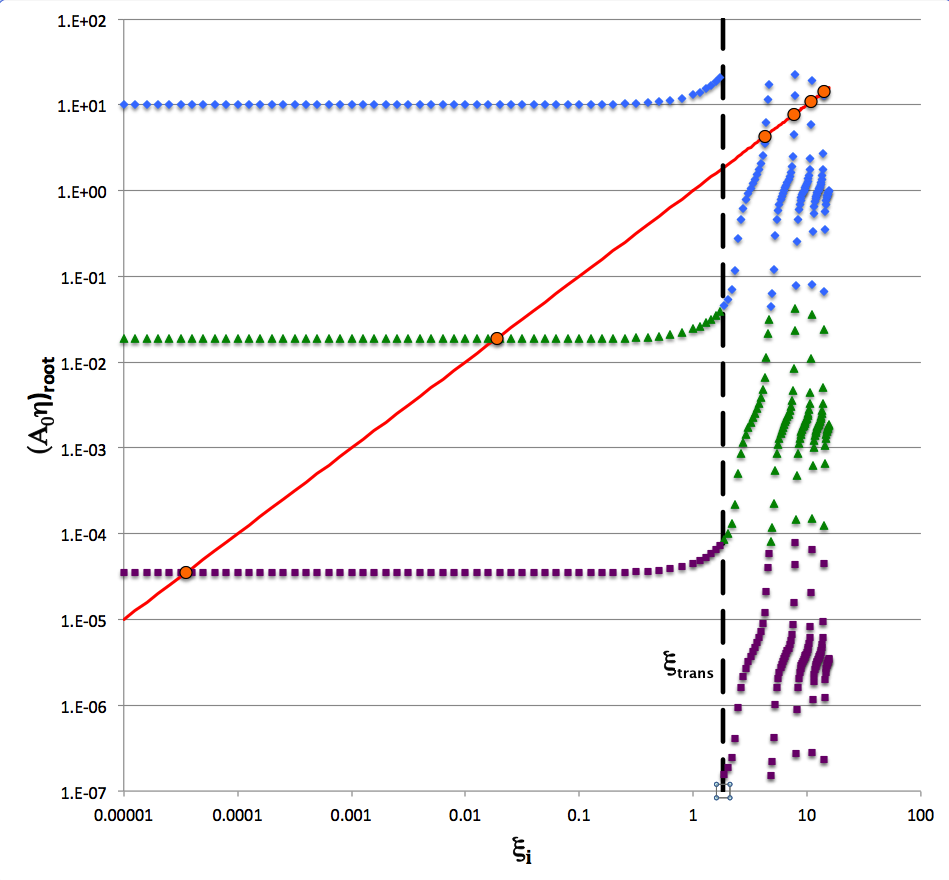
For the case, <math>~\mu_e/\mu_c = 1 \, ,</math> we have determined empirically (to a dozen significant digits), that, <math>~\xi_\mathrm{trans} = 1.836597203152 \, .</math> Just for fun — and, again, for the case, <math>~\mu_e/\mu_c = 1 </math> — we also have determined that <math>~\xi_\mathrm{trans}</math> satisfies the series, <math>~ 0 = \sum_{n=0}^{\infty} (-1)^{n+1} \biggl(\frac{4n+3}{2n+1} \biggr) \frac{\xi_\mathrm{trans}^{2n}}{(2n)!} \, .</math> The black, vertical, long-dashed line in the following figure identifies where <math>~\xi_i = \xi_\mathrm{trans}</math>.
But the one whose value we have determined here is the only one that falls within the physically viable range of interface location values, <math>~0 \le \xi_i \le \pi </math>. |
The following log-log plot shows what value(s) of <math>~(A_0\eta)_\mathrm{root} </math> (vertical axis) result from a wide range of interface coordinate specifications, <math>~\xi_i</math> (horizontal axis), under the simplifying assumption that <math>~(\mu_e/\mu_c) = 1</math>: Solid blue diamonds identify roots resulting from setting <math>~m=0</math> in the phase-shift specification, solid green triangles identify roots for which <math>~m=-1</math>, and solid purple squares identify roots for which <math>~m=-2</math>. As has just been discussed in the context of a cautionary note, as <math>~\xi_i</math> is increased from zero for any given value of <math>~m</math> — that is, as one traverses the plot, moving from the lefthand edge toward the right along a curve of constant color — the solution, <math>~(A_0\eta)_\mathrm{root} </math>, makes an abrupt jump when <math>~\xi_i</math> crosses the value, <math>~\xi_\mathrm{trans}</math>. This identifies the root of the cubic equation for which <math>~\Delta_i = \pi/2 + m\pi</math>. One can continue to move in a smooth, continuous fashion along a single — but multi-colored — solution curve by letting <math>~m \rightarrow (m+1)</math> as <math>~\xi_i</math> crosses <math>~\xi_\mathrm{trans}</math>.
|
Examination of F2 Function Discussed by J. O. Murphy (1983, Proc. Astr. Soc. of Australia, 5, 175) |
||||||||
|
||||||||
The red line in the figure shows where the coordinate value along the vertical axis equals the coordinate value along the horizontal axis. Hence the points where this red line intersects the other curves in the figure can be interpreted as identifying solutions to the cubic equation for which,
<math>~(A_0\eta)_\mathrm{root} = \xi_i \, .</math>
The points of intersection that are highlighted in this figure are also what Murphy (1983) refers to as roots of his <math>~F2 = 0</math> function. The values of ten successive coordinate roots of this function are listed in the right-hand column of Table 1 in Murphy (1983). We have re-listed the values of six of these roots in a column immediately to the right of the above figure and have marked with orange circles the locations of these six points in the figure. As they should, Murphy's identified roots lie precisely at the intersection of the red line with the other curves.
Physically Viable Parameter Values
Interface Mapping
As has already been stated in our above description of the <math>~n_c = 1</math> core of these bipolytropic configurations, the structure of the core will be physically viable as long as the radial location of the interface, <math>~\xi_i</math>, between the core and the envelope is positioned somewhere within the range,
<math>~0 \le \xi_i \le \pi \, .</math>
Similarly, our discussion of Srivastava's Lane-Emden function, which is being used to define the envelope of these bipolytropic configurations, makes it clear that the envelope will have a physically viable structure as long as the parameter, <math>~\Delta_i</math>, associated with the radial location of the interface is positioned somewhere within the range,
<math>~\eta_\mathrm{crit} < e^{2\Delta_i} < e^{2\pi} \, ,</math>
where,
<math>\eta_\mathrm{crit} \equiv e^{2\tan^{-1}(1+2^{1/3})} = 10.05836783\, ,</math>
and, in keeping with the definition provided above,
<math>\Delta_i = \tan^{-1}(y_\mathrm{root}) + m\pi \, .</math>
This coordinate range for the physically viable envelope can be rewritten as,
<math>~\tan^{-1}(1+2^{1/3}) \le \Delta_i \le \pi \, .</math>
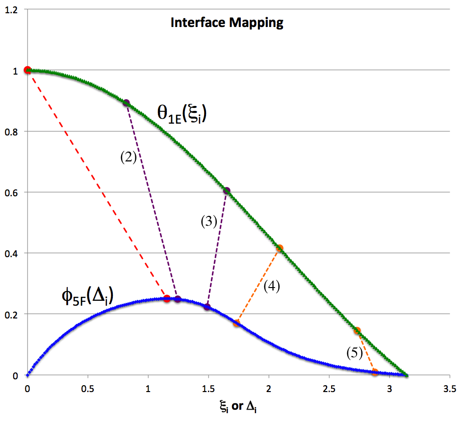
As is illustrated in the following figure, titled "Interface Mapping," our analytic solution defines a smooth, one-to-one mapping of the radial coordinate that defines the outer edge of the <math>~n_c=1</math> core, <math>~\xi_i</math>, to the parameter, <math>~\Delta_i</math>, that defines the inner edge of the <math>~n_e = 5</math> envelope.
|
In the figure, the green curve traces the segment of the E-Type Lane-Emden function for the <math>~n_c = 1</math> polytropic core, <math>~\theta_{1E}</math> — that is, the segment of the "sinc" function — that covers the range <math>~[0,\pi]</math> for the interface parameter, <math>~\xi_i</math>; the blue curve traces the segment of the F-Type Lane-Emden function for the <math>~n_e = 5</math> polytropic envelope, <math>~\phi_{5F}</math>, that covers this same range <math>~[0,\pi]</math>, but for the interface parameter, <math>~\Delta_i</math>. (This blue curve is also displayed, and its properties described in more depth, in a separate discussion devoted to Srivastava's Lane-Emden function for <math>~n=5</math> polytropes.) This entire displayed parameter range, <math>~[0,\pi]</math>, is associated with physically viable interface values for the core (green curve), but for the envelope (blue curve), only a subset of this range can be associated with physically viable interface values — namely, the range <math>~[\tan^{-1}(1+2^{1/3}),\pi]</math> over which <math>~\phi_{5F}</math> is positive but its slope is either negative or zero.
The purple dashed line segment labeled "(2)" in the above "Interface Mapping" figure intersects the green curve at the value, <math>~\xi_i = 0.8154</math>, and it intersects the blue curve at the interface value, <math>~\Delta_i = 1.24287</math>. [These two numerical values are listed in the row labeled "Model (2)" of the table that has been placed immediately to the right of the figure.] This is intended to illustrate that an equilibrium bipolytropic configuration with <math>~(n_c, n_e) = (1, 5)</math> can be constructed by truncating the <math>~n_c = 1</math> core at a radius, <math>~\xi_i = 0.8154</math>, and matching it to an <math>~n_e = 5</math> envelope whose innermost radius is associated with the parameter, <math>~\Delta_i = 1.24287</math>. (The corresponding, analytically determined values of the coefficients <math>~A_0</math> and <math>~B_0</math> dictate the manner in which the blue curve should be stretched both horizontally and vertically to complete a smooth attachment of the envelope to the core.) In an analogous fashion, the dashed line segments labeled "(3)", "(4)", and "(5)" — and their corresponding coordinate values as listed in the accompanying table — illustrate how three additional equilibrium bipolytropic configurations with progressively larger cores can be constructed with the proper interface mapping. We have specifically chosen to illustrate the interface-mapping of these four bipolytropic models because their cores are truncated at the same values of <math>~\xi_i</math> that Murphy (1983) used for the models numbered "(2)", "(3)", "(4)", and "(5)" in his Table 3. (See the much more in-depth discussion, below; and note that the edge of the core is labeled by the parameter, <math>~\zeta_J</math>, rather than by <math>~\xi_i</math>, in Murphy's Table 3.)
For clarity we note that, the analytically determined values of <math>~\Delta_i</math> that are listed in the table that sits to the right of the above "Interface Mapping" figure have been shifted in phase by <math>~m\pi</math>, where the relevant value of the integer, <math>~m</math>, is also listed in the table. In the figure, the two purple dashed-line segments are associated with models for which <math>~m=0</math>, while the two orange dashed-line segments are associated with models for which <math>~m=1</math>.
In his Table 3, Murphy (1983) also tabulates the characteristics of two additional models: The core of his "model 1" is truncated at a radius much less than <math>~\pi</math>, namely, <math>~\xi_i = 0.032678</math>; as a result, the bipolytropic configuration has a very small core and its structure is almost entirely that of an <math>~n = 5</math> polytrope. At the other extreme, the core of his "model 6" is truncated at a radius that is almost, but not quite, equal to <math>~\pi</math>, namely, <math>~\xi_i = 3.1415</math>; the resulting bipolytropic configuration has a very tiny envelope and its structure is almost entirely an <math>~n = 1</math> polytrope. Our analytic solution permits us to set <math>~\xi_i</math> to either of the two limiting values, <math>~0</math> or <math>~\pi</math>, and to show that, in these limits, <math>~\Delta_i</math> exactly equals, respectively, <math>~\tan^{-1}(1 + 2^{1/3})</math> and <math>~\pi</math>. The mapping of the first of these two limits is illustrated by the red dashed line segment in the above figure; the second limit is illustrated simply by the intersection of the two curves at the coordinate location, <math>~\pi</math>. It appears, therefore, that in these two limits Murphy's bipolytrope can be used, respectively, to define the structure of an isolated <math>~n=5</math> polytrope or an isolated <math>~n=1</math> polytrope.
ASIDE: It has previously been thought that Srivastava's Lane-Emden function, <math>~\phi_{5F}</math>, cannot be used on its own to define the structure of an isolated <math>~n=5</math> polytrope because the function's amplitude grows without bound and oscillates more and more rapidly between positive and negative values as the governing radial coordinate gets smaller and smaller. From the results presented here, it now appears as though an isolated <math>~n=5</math> polytrope of this type can be constructed by letting the interface parameter <math>~\xi_i \rightarrow 0</math> — and, hence the alternative parameter <math>~\Delta_i \rightarrow \tan^{-1}(1+2^{1/3})</math> — in Murphy's bipolytrope. It should be interesting to determine the values of the coefficients, <math>~A_0</math> and <math>~B_0</math>, that arise in this limit, and to examine in detail the structure of the complete <math>~n=5</math> model that results. Does its radial density profile resemble — or, perhaps, exactly match — the radial density profile of the well-known isolated <math>~n=5</math> ploytrope? Does the new structure have a finite radius as well as a finite central density? In this context it is worth noting that, in two separate papers — Murphy (1980a) and Murphy (1981) — Murphy has constructed and discussed the physical characteristics of equilibrium models that obey the <math>~n=5</math> polytropic equation of state all the way from the center to a surface which is of finite radius. He accomplishes this by piecing together a core that is defined by the familiar, analytically specified, <math>~\phi_{5E}</math> Lane-Emden function and an envelope that is defined by Srivastava's <math>~\phi_{5F}</math> Lane-Emden function.
Murphy's Example Model Characteristics
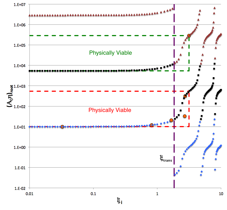
As in an earlier figure, the following log-log plot shows what value(s) of <math>~(A_0\eta)_\mathrm{root} </math> (vertical axis) result from a wide range of interface coordinate specifications, <math>~\xi_i</math> (horizontal axis), under the simplifying assumption that <math>~(\mu_e/\mu_c) = 1</math>. The solid blue diamonds present exactly the same information as in the previous figure, that is, they identify roots resulting from setting <math>~m=0</math> in the phase-shift specification. But here, focusing on a regime that highlights larger roots of the first constraint equation, solid black squares identify roots for which <math>~m=+1</math>, and solid maroon triangles identify roots for which <math>~m=+2</math>.
In this version of the figure, colored dashed-line segments have been drawn to enclose two regions of parameter space in which solutions of the key nonlinear interface relation produce a physically viable model — that is, <math>~0 \le \xi_i \le \pi</math> and <math>~\tan^{-1}(1+2^{1/3}) \le \Delta_i \le \pi</math>. The portion of the red-outlined rectangular region that lies to the left of the vertical, <math>~\xi_i = \xi_\mathrm{trans}</math> line accommodates some models that arise from specifying an <math>~m=0</math> phase shift and the portion that lies to the right of this demarcation line accommodates some models that arise from specifying an <math>~m=+1</math> phase shift. Similarly, the portion of the green-outlined rectangular region that lies to the left of the vertical, <math>~\xi_i = \xi_\mathrm{trans}</math> line accommodates additional models that arise from specifying an <math>~m=+1</math> phase shift and the portion that lies to the right of this demarcation line accommodates models that arise from specifying an <math>~m=+2</math> phase shift. Given the inherent periodicity of Srivastava's <math>~\phi_{5F}</math> function, it should be clear that we could equally well have identified other rectangular regions at both higher <math>~(m \ge 2)</math> and lower <math>~(m \le 0)</math> values of <math>~(A_0 \eta)_\mathrm{root}</math> in which additional physically viable models exist. It should also be clear that, because the figure presents a log-log plot and the lower limit of viable parameter values for the horizontal axis parameter, <math>~\xi_i</math>, is zero, the identified rectangular regions should be viewed as extending to the left, all the way to minus infinity.
|
Examination of Table 3 Data Presented in J. O. Murphy (1983, Proc. Astr. Soc. of Australia, 5, 175) |
|||||||||||||||||
|
|||||||||||||||||
In his Table 3, Murphy (1983) presents six pairs of "coordinate" roots, <math>~(\zeta_J, \xi_J)</math>, that not only satisfy the first constraint equation but that also, in his interpretation, identify physically viable model solutions. The values of all six of these coordinate pairs have been re-listed immediately to the right of the log-log plot, in a separate panel of the above figure. After mapping Murphy's coordinate notation to ours — specifically invoking the mapping <math>~(\zeta_J, \xi_J) ~\rightarrow~ (\xi_i, A_0\eta_\mathrm{root})</math> — the locations of all six models have been marked by orange circles on the plot. Five of Murphy's models fall directly onto our generated curves and in regions marked as physically viable, giving us confidence that our analysis matches his in considerable detail. As is explained more fully, below, we strongly suspect that the single Murphy model that does not lie on one of our generated curves — "Model 4" which, as published in Murphy's Table 3, has coordinates <math>~(\zeta_J, \xi_J) = (2.6914, 33.0249)</math> — is displaced, perhaps because of transcription errors in the published table.
As a supplement to the preceding two figures, we now display a table of our analytically determined model characteristics that is patterned after and largely matches Murphy's (1983) Table 3. The tabulated values have been derived assuming <math>~\mu_e/\mu_c = 1</math> throughout, that is, assuming that the mean molecular weights of the core and the envelope are identical. Vertically, the table is divided into three segments: The top portion contains six rows of numbers that result from our derivations; the middle portion displays six columns of numbers that have been extracted directly from Table 3 of Murphy (1983) and displayed here as image segments; and the bottom portion shows additional parameter values that we have generated in an effort to understand why our "Model 4" does not match the fourth model in Murphy's table.
|
Some Model Characteristics† (assuming <math>\mu_e/\mu_c</math> = 1) |
||||||||
|
Model |
Specified |
Analytically Determined Here |
||||||
|
<math>~\xi_i</math> |
<math>~m</math> |
<math>~\Delta_i</math> |
<math>~(A_0\eta)_\mathrm{root}</math> |
<math>~\frac{A_0}{3^{1/2}} \biggl( \frac{\mu_e}{\mu_c} \biggr) </math> |
<math>~B_0</math> |
<math>~\frac{B_0}{3^{1/4}} \biggl(\frac{\mu_e}{\mu_c}\biggr)^{1/2} \theta_i^{-1} </math> |
<math>~\xi_s</math> |
|
| 1 | 3.2678E-02 | 0 | 1.1544 | 10.0614 | 307.894 | 5.77929 | 4.39209 | 1.7392 |
| 2 | 0.8154 | 0 | 1.2429 | 12.0101 | 14.729 | 1.25567 | 1.06865 | 36.356 |
| 3 | 1.6598 | 0 | 1.4918 | 19.7585 | 11.9041 | 1.01206 | 1.28146 | 44.984 |
| 4 | 2.6914 | 1 | 2.8365 | 290.9431 | 108.1010 | 0.14348 | 0.67430 | 4.9536 |
| 5 | 2.7302 | 1 | 2.8749 | 100.00<math>\pi</math> | 115.065 | 0.12408 | 0.64370 | 4.6539 |
| 6 | 3.1415 | 2 | 6.283141 | 91268<math>\pi</math> | 170.44223<math>e^{2\pi}</math> | 1.8966E-05 | 0.48862 | 3.141778 |
|
Corresponding Values Extracted Directly from Murphy's (1983) Table 3 |
||||||||
 |
||||||||
|
Attempting to Understand Murphy's "Model 4" |
||||||||
| 4b | 0.048681 | 0 | 1.1545342 | 10.065043 | 206.75505 | 4.7358862 | 3.5999 | 2.589981 |
| 4c | 1.14988 | 0 | 1.3234244 | 14.109506 | 12.2704 | 1.12444163 | 1.07640071 | 43.6409 |
| 4d | 1.77027 | 0 | 1.5391618 | 21.721958 | 12.2704 | 0.9876639 | 1.355397 | 43.6409 |
| 4e | 2.10961 | 1 | 1.7486314 | 33.0249 | 15.6545186 | 0.8651536 | 1.6157228 | 34.2068427 |
|
†See an accompanying discussion for a complementary critique of Murphy's Table 3 models including an evlauation of the functions, <math>~U_{1E}</math>, <math>~V_{1E}</math>, <math>~U_{5F}</math>, and <math>~V_{5F} \, .</math> |
||||||||
Our six models (top portion of the above table) have been constructed by, first, specifying the location of the outer edge of the core, <math>~\xi_i</math> along with a corresponding phase shift parameter, <math>~m</math>, to match Murphy's chosen core-interface values — in his terminology, <math>~\zeta_J</math> (middle portion of the above table). Once the value of <math>~\xi_i</math> has been specified for each model, the value of the parameter, <math>~p</math>, the root of the cubic equation, <math>~y_\mathrm{root}</math>, and all of the parameter values listed in the upper portion of the table were determined using the parameter relations derived above and/or detailed in the table below. For example,
|
<math>~\Delta_i</math> |
<math>~=</math> |
<math>~\tan^{-1}(y_\mathrm{root}) + m\pi \, ;</math> |
|
<math>~(A_0\eta)_\mathrm{root}</math> |
<math>~=</math> |
<math>~e^{2\Delta_i} \, ;</math> |
and,
|
<math>~\xi_s</math> |
<math>~=</math> |
<math>~\xi_i e^{2(\pi -\Delta_i)} \, .</math> |
Comparing our tabulated numbers (upper portion of the table) with the numbers published by Murphy (middle portion of the table) adds strong support to the statement made in connection with the above figure, that is, that our analysis matches Murphy's in considerable detail. But such a comparison also highlights the mismatch between Murphy's "Model 4" and ours — to aid in this particular comparison, the relevant numbers have been displayed in a red font in the upper portion of our table. According to our analysis, a model with <math>~\xi_i = 2.6914</math> does not display characteristics that, in any fashion, match Murphy's model with the same core-interface value.
We initially suspected that the "Model 4" mismatch resulted from a typographical or transcription error in the value of <math>~\zeta_J</math> — in our terminology, <math>~\xi_i</math> — that appears in Murphy's published Table 3. So we tried a variety of values of <math>~\xi_i</math>, looking for a set of generated characteristics that matched Murphy's published Model 4 characteristics. We were unsuccessful in this effort. The most tantalizing results from this search are displayed as cells with light-green backgrounds in the bottom segment of the above table: (Model 4b) Setting <math>~\xi_i = 0.048681~(m = 0)</math> gives <math>~B=3.5999</math>, which matches Murphy's "Model 4" value of <math>~B</math>; (Model 4c) setting <math>~\xi_i = 1.14988~(m = 0)</math> gives values of <math>~A</math> and <math>~\zeta_J (\mathrm{i.e.,}~\xi_s)</math> that both match Murphy's values; (Model 4d) setting <math>~\xi_i = 1.77027~(m = 0)</math> also gives values of <math>~A</math> and <math>~\zeta_J</math> that both match Murphy's values; and (Model 4e) setting <math>~\xi_i = 2.10961~(m = 1)</math> gives a value of <math>~(A_0\eta)_\mathrm{root}</math> that matches Murphy's value of <math>~\xi_J</math>. As we have been unable to find a value of <math>~\xi_i</math> whose associated parameter values match Murphy's "Model 4" values across the board, we remain at a loss to explain the mismatch between our "Model 4" and Murphy's.
Step 8: Envelope's Physical Profile
Combining the set of expressions provided in the right-most column of the accompanying bipolytrope "Table 1: Setup" with the interface conditions already established, above, we can now specify how the density, pressure, and integral mass vary throughout the envelope, that is, over the radial extent <math>\xi_i \le \xi \le \xi_s</math>.
|
<math>~\rho</math> |
<math>~=</math> |
<math>~\rho_e \phi^{5}</math> |
|
|
<math>~=</math> |
<math>~\rho_0 \biggl( \frac{\mu_e}{\mu_c} \biggr) \theta_i \phi^{5} \, ;</math> |
|
<math>~P</math> |
<math>~=</math> |
<math>~K_e \rho_e^{6/5} \phi^{6}</math> |
|
|
<math>~=</math> |
<math>~K_c \biggl[\rho_0^{4}\biggl( \frac{\mu_e}{\mu_c} \biggr)^{-6} \theta^{4}_i\biggr]^{1/5} \biggl[ \rho_0 \biggl( \frac{\mu_e}{\mu_c} \biggr) \theta_i \biggr]^{6/5} \phi^{6}</math> |
|
|
<math>~=</math> |
<math>~K_c \rho_0^2 \theta^{2}_i \phi^{6} \, ;</math> |
|
<math>~M_r</math> |
<math>~=</math> |
<math>~4\pi \biggl[ \frac{3K_e}{2\pi G} \biggr]^{3/2} \rho_e^{-1/5} \biggl(-\eta^2 \frac{d\phi}{d\eta} \biggr)</math> |
|
|
<math>~=</math> |
<math>~\biggl[ \frac{3^3 \cdot (2^2\pi)^2}{2^3\pi^3 G^3} \biggr]^{1/2} \biggl[K_c^5 \rho_0^{4}\biggl( \frac{\mu_e}{\mu_c} \biggr)^{-6} \theta^{4}_i\biggr]^{3/10} \biggl[ \rho_0 \biggl( \frac{\mu_e}{\mu_c} \biggr) \theta_i \biggr]^{-1/5} \biggl(-\eta^2 \frac{d\phi}{d\eta} \biggr)</math> |
|
|
<math>~=</math> |
<math>~\biggl[ \frac{2\cdot 3^3 }{\pi G^3} \biggr]^{1/2} K_c^{3/2} \rho_0 \theta_i \biggl( \frac{\mu_e}{\mu_c} \biggr)^{-2} \biggl(-\eta^2 \frac{d\phi}{d\eta} \biggr) \, .</math> |
Examples
Normalization
The dimensionless variables used in Tables 1 & 2 are defined as follows:
|
<math>~\rho^*</math> |
<math>~\equiv</math> |
<math>~\frac{\rho}{\rho_0}</math> |
; |
<math>~r^*</math> |
<math>~\equiv</math> |
<math>~\frac{r}{(K_c/G)^{1/2}}</math> |
|
<math>~P^*</math> |
<math>~\equiv</math> |
<math>~\frac{P}{K_c\rho_0^{2}}</math> |
; |
<math>~M_r^*</math> |
<math>~\equiv</math> |
<math>~\frac{M_r}{\rho_0 (K_c/G)^{3/2}}</math> |
|
<math>~H^*</math> |
<math>~\equiv</math> |
<math>~\frac{H}{K_c\rho_0}</math> |
. |
|
||
Parameter Values
The <math>2^\mathrm{nd}</math> column of Table 1 catalogues the analytic expressions that define various parameters and physical properties (as identified, respectively, in column 1) of the <math>~n_c=1</math>, <math>~n_e=5</math> bipolytrope.
|
Properties of <math>~n_c=1</math>, <math>~n_e=5</math>, BiPolytrope Having Various Interface Locations, <math>~\xi_i</math> |
|
|
Parameter |
<math>~\xi_i</math> |
|
<math>~\theta_i</math> |
<math>~\frac{\sin\xi_i}{\xi_i} </math> |
|
<math>~-\biggl(\frac{d\theta_i}{d\xi}\biggr)_i</math> |
<math>~\frac{1}{\xi_i^2}(\sin\xi - \xi_i \cos\xi_i) </math> |
|
<math>~r^*_\mathrm{core} \equiv r^*_i</math> |
<math>~\biggl( \frac{1}{2\pi} \biggr)^{1/2} \xi_i</math> |
|
<math>~\rho^*_i \biggr|_c = \biggl( \frac{\mu_e}{\mu_c} \biggr)^{-1} \rho^*_i \biggr|_e</math> |
<math>~\theta_i</math> |
|
<math>P^*_i</math> |
<math>~\theta_i^2</math> |
|
<math>H^*_i \biggr|_c = \frac{n_c+1}{n_e+1} \biggl( \frac{\mu_e}{\mu_c} \biggr) H^*_i \biggr|_e</math> |
<math>~2\theta_i</math> |
|
<math>M^*_\mathrm{core}</math> |
<math>~\biggl( \frac{2}{\pi} \biggr)^{1/2} (\sin\xi_i - \xi_i \cos\xi_i)</math> |
|
<math>\biggl( \frac{\mu_e}{\mu_c} \biggr)^{-1}\eta_i</math> |
<math>\frac{\xi_i}{\sqrt{3}}</math> |
|
<math>~ -\biggl( \frac{d\phi}{d\eta} \biggr)_i</math> |
<math>~\frac{1}{\sqrt{3} \theta_i}\biggl( - \frac{d\theta}{d\xi} \biggr)_i = \frac{1}{\sqrt{3}}\biggl( \frac{1}{\xi_i}- \cot\xi_i\biggr)</math> |
|
<math>~p</math> |
<math>~\frac{3}{ 3-2(\mu_e/\mu_c)(1-\xi_i \cot\xi_i)}</math> |
|
<math>~~y_\mathrm{root}</math> |
<math>~p\biggl( 1 + \{1 + [1 + (p^{-2}-1)^3]^{1/2}\}^{1/3} + \{1 - [1 + (p^{-2}-1)^3]^{1/2}\}^{1/3} \biggr)</math> |
|
<math>~\Delta_i - m\pi</math> |
<math>~\tan^{-1}(y_\mathrm{root})</math> |
|
<math>~(A_0\eta)_\mathrm{root}</math> |
<math>~e^{2\Delta_i}</math> |
|
<math>~\xi_s</math> |
<math>~\xi_ie^{2(\pi-\Delta_i)}</math> |
|
<math>~\biggl[ \frac{A_0}{3^{1/2}} \biggl( \frac{\mu_e}{\mu_c} \biggr) \biggr]</math> |
<math>~\xi_i^{-1} e^{2\Delta_i}</math> |
|
<math>~\biggl[\frac{B_0}{3^{1/4}} \biggl( \frac{\mu_e}{\mu_c} \biggr)^{1/2} \biggr]</math> |
<math>~\biggl[ \xi_i \biggl( \frac{3}{\sin^2\Delta_i} - 2\biggr) \biggr]^{-1/2} = \theta_i \biggl[ \frac{\xi_i^{1/2}}{\sin\xi_i}\biggl( \frac{3}{\sin^2\Delta_i} - 2\biggr)^{-1/2} \biggr] </math> |
|
<math>~ -\biggl( \frac{d\phi}{d\eta} \biggr)_s \biggl( \frac{\mu_e}{\mu_c}\biggr)</math> |
<math>~\frac{1}{ 2\xi_i e^{3(\pi-\Delta_i)}} \biggl( \frac{3}{\sin^2\Delta_i} - 2 \biggr)^{1/2}</math> |
|
<math>~ R^*_s</math> |
<math>~(2\pi)^{-1/2} \xi_i e^{2(\pi - \Delta_i)}</math> |
|
<math>~ \biggl( \frac{\mu_e}{\mu_c}\biggr) M^*_\mathrm{tot}</math> |
<math>~\biggl( \frac{3}{2\pi} \biggr)^{1/2} \sin\xi_i \biggl( \frac{3}{\sin^2\Delta_i} - 2 \biggr)^{1/2} e^{(\pi - \Delta_i)}</math> |
Profile
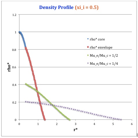
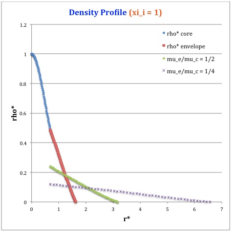
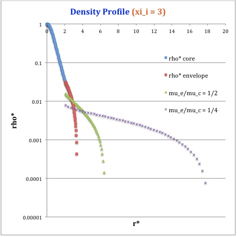
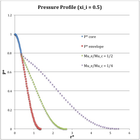
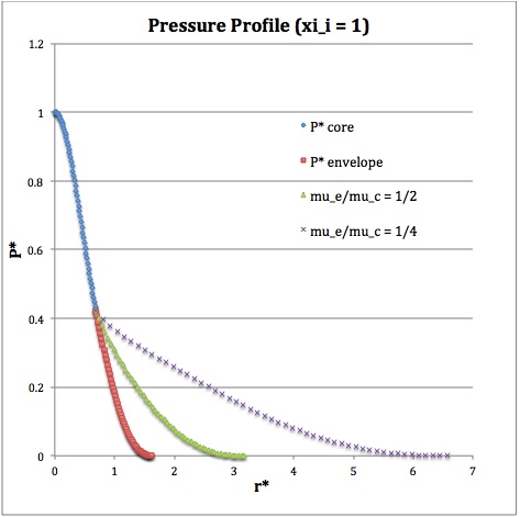
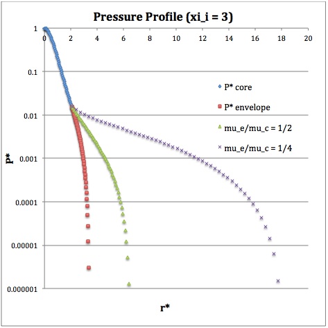
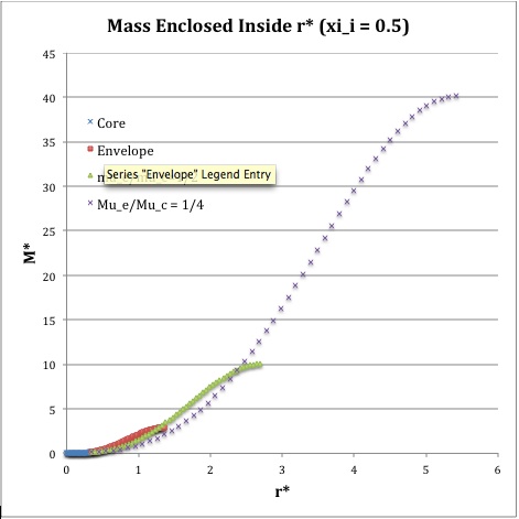
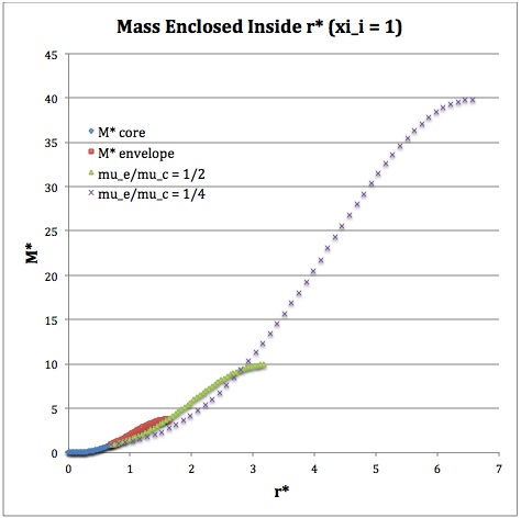
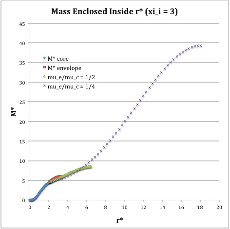
Once the values of the key set of parameters have been determined as illustrated in the preceding formula table, the radial profile of various physical variables can be determined throughout the bipolytrope as detailed in step #4 and step #8, above. The following table summarizes the mathematical expressions that define the profile throughout the core (column 2) and throughout the envelope (column 3) of the normalized mass density, <math>~\rho^*(r^*)</math>, the normalized gas pressure, <math>~P^*(r^*)</math>, and the normalized mass interior to <math>~r^*</math>, <math>~M_r^*(r^*)</math>. For all profiles, the relevant normalized radial coordinate is <math>~r^*</math>, as defined in the 2nd row of the table. Graphical illustrations of these resulting profiles can be viewed by clicking on the thumbnail images posted in the last few columns of the table.
Table 2: Radial Profile of Various Physical Variables
|
Variable |
Throughout the Core |
Throughout the Envelope† |
Plotted Profiles |
||
|
<math>\xi_i = 0.5</math> |
<math>\xi_i = 1.0</math> |
<math>\xi_i = 3.0</math> |
|||
|
<math>~r^*</math> |
<math>\biggl( \frac{1}{2\pi} \biggr)^{1/2} \xi</math> |
<math>\biggl( \frac{\mu_e}{\mu_c} \biggr)^{-1} \biggl(\frac{3}{2\pi}\biggr)^{1/2}\eta</math> |
|
||
|
<math>~\rho^*</math> |
<math>\frac{\sin\xi}{\xi}</math> |
<math>\biggl( \frac{\mu_e}{\mu_c} \biggr) \theta_i [\phi(\eta)]^5</math> |
|||
|
<math>~P^*</math> |
<math>\biggl( \frac{\sin\xi}{\xi} \biggr)^2</math> |
<math>\theta^{2}_i [\phi(\eta)]^{6}</math> |
|||
|
<math>~M_r^*</math> |
<math>\biggl( \frac{2}{\pi}\biggr)^{1/2} (\sin\xi - \xi\cos\xi)</math> |
<math>\biggl( \frac{\mu_e}{\mu_c} \biggr)^{-2} \biggl( \frac{2\cdot 3^3 }{\pi} \biggr)^{1/2} \theta_i \biggl(-\eta^2 \frac{d\phi}{d\eta} \biggr) </math> |
|||
|
†In order to obtain the various envelope profiles, it is necessary to evaluate <math>~\phi(\eta)</math> and its first derivative using the information presented in Step 6, above. |
|||||
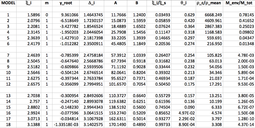
Murphy and Fiedler (1985)
|
Table 1 from Murphy & Fiedler (1985, Proc. Astr. Soc. of Australia, 6, 219) |
|
Reproduction of Table 1 from MF85 Using Excel and Analytic Expressions Derived Here |
Key References
- S. Srivastava (1968, ApJ, 136, 680) A New Solution of the Lane-Emden Equation of Index n = 5
- H. A. Buchdahl (1978, Australian Journal of Physics, 31, 115): Remark on the Polytrope of Index 5 — the result of this work by Buchdahl has been highlighted inside our discussion of bipolytropes with <math>~(n_c, n_e) = (5, 1)</math>.
- J. O. Murphy (1980a, Proc. Astr. Soc. of Australia, 4, 37): A Finite Radius Solution for the Polytrope Index 5
- J. O. Murphy (1980b, Proc. Astr. Soc. of Australia, 4, 41): On the F-Type and M-Type Solutions of the Lane-Emden Equation
- J. O. Murphy (1981, Proc. Astr. Soc. of Australia, 4, 205): Physical Characteristics of a Polytrope Index 5 with Finite Radius
- J. O. Murphy (1982, Proc. Astr. Soc. of Australia, 4, 376): A Sequence of E-Type Composite Analytical Solutions of the Lane-Emden Equation
- J. O. Murphy (1983, Australian Journal of Physics, 36, 453): Structure of a Sequence of Two-Zone Polytropic Stellar Models with Indices 0 and 1
- J. O. Murphy (1983, Proc. Astr. Soc. of Australia, 5, 175): Composite and Analytical Solutions of the Lane-Emden Equation with Polytropic Indices n = 1 and n = 5
- J. O. Murphy & R. Fiedler (1985a, Proc. Astr. Soc. of Australia, 6, 219): Physical Structure of a Sequence of Two-Zone Polytropic Stellar Models
- J. O. Murphy & R. Fiedler (1985b, Proc. Astr. Soc. of Australia, 6, 222): Radial Pulsations and Vibrational Stability of a Sequence of Two-Zone Polytropic Stellar Models
Related Discussions

|
|---|
|
© 2014 - 2021 by Joel E. Tohline |

