Discussing Patrick Motl's 2019 Simulations

May 1 (from Patrick)

Hi Joel,

I hope things are well for you and yours.

I did finally have a couple research students this semester that were able to slog their way into unix, programming, etc. far enough to do some useful things.

They ran two spherical bipolytropes with my old cylindrical code. These were n = 5 cores with n = 1 envelopes. No density discontinuity. One model is a little below the stability boundary in xi, the other is a little above the stability boundary.

What I can see from the evolutions, especially now that I made plots of the entropy, is that they are convectively unstable and that is just a mess with the core convecting into the envelope.

Did you happen to have any thoughts on what might be a better case to run? When I get done grading finals I am going to work through the equations with kappa set explicitly in the envelope so the entropy profile is flat and just live with whatever density discontinuity that gives me.

cheers, Patrick

May 4 (from Joel)

Patrick,

My initial response to your 1 May email follows. In an effort to make sure we are on the same page when referencing the structural properties and the stability properties of various configurations, my response includes links to various chapters/subsections of my online wiki-based book.

Thanks for pursuing this problem. I am still very interested in Its solution.

All the best, Joel

Chosen Initial Models

I presume that when you constructed your pair of initial (spherical) models, you used the analytically prescribed properties found in my chapter titled, "BiPolytrope with <math>n_c = 5</math> and <math>n_e=1</math>" and that when you reference the "stability boundary in <math>~\xi</math>" you are drawing from the summary (Table 3 and Figure 3) found near the end of this chapter in the subsection titled, "Stability Condition." In particular, based on the information contained in this chapter, I presume that you are assuming that the marginally unstable model along the <math>~\mu_e/\mu_c = 1</math> sequence is the configuration having the properties …

and that your pair of initial models have values of <math>~\xi_i</math> that are somewhat greater than and somewhat smaller than 2.416. If this does not properly describe your choice of initial models, please clarify.

Instability Toward Convection

In my chapter titled, "Axisymmetric Instabilities to Avoid," I discuss — among other things — the Schwarzschild Criterion. Toward the very end of that chapter, in a subsection titled, Modeling Implications and Advice, I specifically describe how convection might arise when modeling spherical polytropic configurations. Would you please read this short subsection and let me know whether you agree with my explanation or not?

In the context of this discussion of the Schwarzschild criterion (i.e., convective instabilities) in polytropes, my question to you is: What value of the adiabatic index, <math>~\gamma</math>, did you use when you evolved the bipolytrope? Did you use the same index for the entire configuration, or did you use a value in the envelope that is different from the value used in the core?

If you used <math>~\gamma = 6/5</math> for the core, then the core should have uniform specific entropy and therefore would be (only) marginally stable against convection. Likewise, if you used <math>~\gamma = 2</math> for the envelope, it should be (only) marginally stable against convection. Incidentally, these are the two separate values of the adiabatic index that I used when I used a free-energy analysis to examine stability.

NOTE: In yet another chapter of my book, I discuss the bipolytropic stability analysis that was performed by Murphy & Fiedler (1985b). They examined the stability of bipolytropes having the core/envelope polytropic indexes swapped, that is, their equilibrium models had, <math>~(n_c, n_e) = (1, 5)</math>. Their stability analysis was performed while assuming that the adiabatic index was <math>~\gamma = 5/3</math> throughout the entire configuration. In a short subsection near the beginning of my chapter titled, "Aside Regarding Convectively Unstable Core," I have pointed out that the cores of these models should have all been convectively unstable, according to the Schwarzschild criterion. Please read this short subsection and let me know if you agree with my stated expectation for those models.

Other Approaches to Stability Analysis

After you send me feedback on the comments & questions I have presented, above, I have a good deal more to tell you about my analysis of the stability of our <math>~(n_c, n_e) = (5, 1)</math> bipolytropic configurations. I am still a bit confused, but I'm pretty sure that the transition from stable to unstable configurations along the <math>~\mu_e/\mu_c = 1</math> occurs at a value of <math>~\xi_i \approx 1.67</math>, rather than the value of <math>~\xi_i = 2.416</math> that I obtained via the free-energy analysis. But, as I've said, there is a lot to tell you about this.

Other Suggestions

You asked what alternative models might be examined. It might be smarter to first evolve some simpler models, such as pressure-truncated polytropes — not bipolytropes. But we should discuss this after I read your feedback on the above.

May 4 (from Patrick)

Hi Joel,

Replying to your web page

The models have xi_interface values of 2.39184 and 2.44016

For the evolutions, I used passive scalars to identify fluids as core or envelope and use effective polytropic indices and exponents based on the proportion of the fluid in a given cell that is core or envelope.

There is slightly more to it than that as the “vacuum” is n = 1.5 and a third fluid type.

When I do that, the stars are definitely convectively unstable.

s.ps is a quick plot of entropy vs radial cell number. The fluid in the envelope is lower in entropy than fluid in the core.

The entropy plotted is c_p ln( tau / rho) = R (gamma/(gamma-1)) ln (tau / rho) where R is the gas constant.

The movie shows the meridional cross section of density through the star, the core envelope boundary corrugates pretty quickly in the run and then everything goes off the rails. There may be more than one problem but the convective instability is definitely one problem.

cheers, Patrick

May 5 (following a phone conversation with Patrick)

Tying Expressions into H_Book Context

In our wiki-based chapter titled, "First Law of Thermodynamics," we have introduced the concept of an entropy tracer, <math>~\tau</math>. In the subsubsection of this chapter that is titled, "Substantiation," we show that an expression for the specific entropy of a fluid element is,

<math>~s = c_P \ln\biggl( \frac{\tau}{\rho} \biggr) + \mathrm{constant} \, .</math>

In addition, from our wiki-based chapter titled, "Ideal Gas Equation of State," we find the relations,

and,

<math>~\gamma_g </math>

<math>~\Rightarrow</math>

<math>~\frac{\gamma_g}{(\gamma_g-1)} \biggl( \frac{\Re}{\bar\mu} \biggr) \, .</math>

Hence this expression for the entropy may be rewritten as,

<math>~s = \frac{\gamma_g}{\gamma_g-1} \biggl( \frac{\Re}{\bar\mu} \biggr) \ln\biggl( \frac{\tau}{\rho} \biggr) + \mathrm{constant} \, .</math>

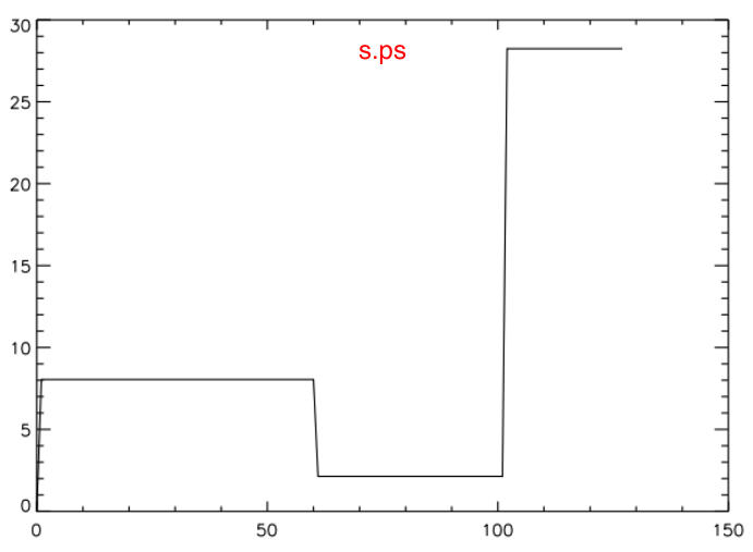
Aside from the factor of <math>~({\bar\mu})^{-1}</math> that appears on the RHS — more on this later — these are the expressions that Patrick has used to generate the s.ps plot, where the (unlabeled) ordinate is the normalized specific entropy, <math>~s/\Re</math>.

At the end of another subsubsection titled, "Initial Recognition," we also find a relevant expression, namely,

<math>~\tau \equiv (\rho\epsilon)^{1/\gamma_g} = \biggl[ \frac{P}{(\gamma_g - 1)} \biggr]^{1/\gamma_g} \, .</math>

Hence, ignoring the additive constant, in general we may write,

<math>~\frac{s}{\Re/\bar{\mu}}</math>	<math>~=</math>	<math>~ \frac{1}{(\gamma_g-1)}\ln \biggl(\frac{\tau}{\rho}\biggr)^{\gamma_g} </math>
	<math>~=</math>	<math>~ \frac{1}{(\gamma_g-1)}\ln \biggl[ \frac{P}{(\gamma_g-1)\rho^{\gamma_g}} \biggr] \, . </math>

Understanding the Step Function at the Core-Envelope Interface

Now, turning to the accompanying tabular summary of the Radial Profile of Various Physical Variables, we are able to determine how the specific entropy behaves throughout the core and, separately, throughout the envelope in <math>~(n_c, n_e) = (5, 1)</math> bipolytropes.

CORE: Throughout the core, we see that,

<math>~\biggl(1+ \frac{\xi^2}{3}\biggr)^{-3}</math>

and

<math>~\biggl(1+ \frac{\xi^2}{3}\biggr)^{-5/2}</math>

and

<math>~\gamma_g</math>

Hence, independent of the radial location, <math>~\xi</math>, throughout the core,

<math>~\frac{s}{\Re/\bar{\mu}}\biggr|_\mathrm{core}</math>

ENVELOPE: Throughout the envelope, we see that,

<math>~\theta_i^6 [\phi(\eta)]^2</math>

and

<math>~\biggl(\frac{\mu_e}{\mu_c}\biggr)\theta_i^5 [\phi(\eta)]</math>

and

<math>~\gamma_g</math>

Hence, independent of the radial location, <math>~\eta</math>, throughout the envelope,

<math>~\frac{s}{\Re/\bar{\mu}}\biggr|_\mathrm{env}</math>

<math>~ \ln \biggl[ \biggl(\frac{\mu_e}{\mu_c}\biggr)^{-2} \theta_i^{-4} \biggr] </math>

<math>~ \ln \biggl[ \biggl(\frac{\mu_e}{\mu_c}\biggr)^{-2} \biggl( 1 + \frac{\xi_i^2}{3}\biggr)^2 \biggr] \, . </math>

It is therefore clear that the core is a uniform specific-entropy sphere and the envelope is a uniform specific-entropy spherical shell, but in general the specific entropy of material in the envelope is different from the specific entropy of material in the core.

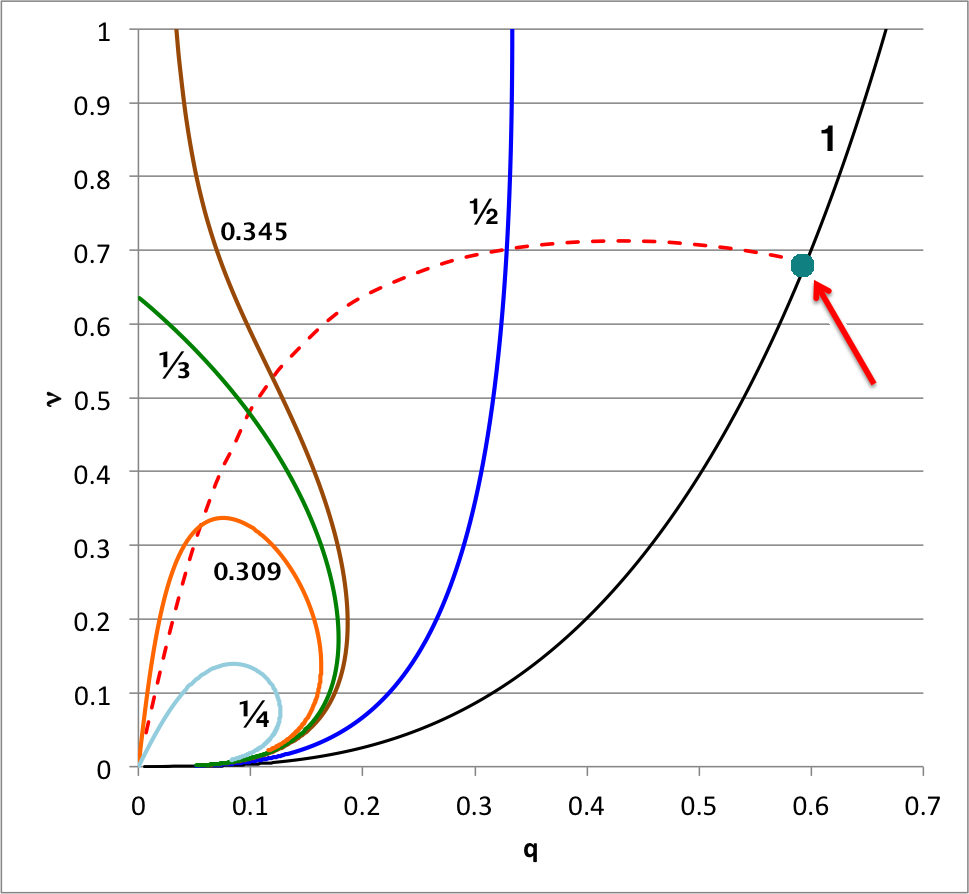
According to our free-energy based evaluation of the stability of bipolytropes having <math>~(n_c, n_e) = (5, 1)</math>, the marginally unstable model along the <math>~\mu_e/\mu_c = 1</math> sequence has the following properties: <math>~(\xi_i, q, \nu, \rho_c/\bar\rho) = (2.41610822, 0.59520261, 0.68306067, 16.3788)</math>; the red arrow in the following diagram points to this model's position in the <math>~q-\nu</math> parameter plane. In an effort to test whether or not this model does identify the transition from stable to unstable configurations along the <math>~\mu_e/\mu_c = 1</math> sequence, Patrick picked a pair of models (highlighted in green in the following table) that straddle the location of the marginally unstable model, and followed the dynamical evolution of both models using a fully 3-D hydrodynamics code. In particular, for the pair of models that Patrick evolved, we find:

Initial Model Parameters for Patrick's Pair of Simulations (green background)
<math>~\frac{\mu_e}{\mu_c}</math>	<math>~\xi_i</math>	<math>~\frac{s}{\Re/\bar{\mu}}\biggr\|_\mathrm{core}</math>	<math>~\frac{s}{\Re/\bar{\mu}}\biggr\|_\mathrm{env}</math>
1	2.39184	8.04719	2.13422
1	2.41610822	8.04719	2.16080
1	2.44016	8.04719	2.18706

For more details, see the accompanying discussion titled, Free-Energy Stability Evaluation

These tabulated values of the normalized specific entropy in the core and, separately, in the envelope appear to be consistent with Patrick's s.ps plot of specific entropy. In particular, this confirms that a step function should appear at the core-envelope interface and that the specific entropy of the envelope material should be lower than the specific entropy of the core material. Therefore, the Schwarzschild criterion is violated at the interface and we should not have been surprised to see convective motions develop — initially, only at the interface.

Can the Step Function be Flipped or Erased

Assume a Mean-Molecular-Weight Ratio of Unity

If we continue to examine equilibrium models that have <math>~\mu_e/\mu_c = 1</math>, is there a value of the interface radius, <math>~\xi_i</math>, for which the entropy step-function disappears and above which the step function flips? The answer appears to be, "Yes." It occurs along the equilibrium sequence where the normalized specific entropy has the same value in the core and as in the envelope. That is, it occurs when,

<math>~ \ln \biggl[ \biggl( 1 + \frac{\xi_i^2}{3}\biggr)^2 \biggr]_\mathrm{smooth} </math>	<math>~=</math>	<math>~5\ln(5)</math>
<math>~ \Rightarrow ~~~ \biggl( 1 + \frac{\xi_i^2}{3}\biggr)_\mathrm{smooth} </math>	<math>~=</math>	<math>~5^{5 / 2}</math>
<math>~ \Rightarrow ~~~ [\xi_i ]_\mathrm{smooth} </math>	<math>~=</math>	<math>~\biggl[3 \biggl(5^{5 / 2} - 1 \biggr)\biggr]^{1 / 2} \approx 12.83375</math> …

Prediction: Any initial model with <math>~\mu_e/\mu_c = 1</math> and <math>~\xi_i > [\xi_i]_\mathrm{smooth}</math> will be stable against convection, but will be globally dynamically unstable.

Pick a Different Molecular-Weight Ratio

In principle, we can determine in a similar fashion the values of <math>~[\xi_i]_\mathrm{smooth}</math> that are relevant to equilibrium model sequences having <math>~\mu_e/\mu_c < 1</math>. But in doing this, we must take into account that in most of our above derivations the mean-molecular-weight appears in the denominator of the (LHS) expression for the normalized specific entropy. More generally, the prescription for <math>~[\xi_i]_\mathrm{smooth}</math> should come from the demand that,

<math>~0</math>	<math>~=</math>	<math>~\frac{s_\mathrm{env}}{\Re} - \frac{s_\mathrm{core}}{\Re}</math>
<math>~\Rightarrow ~~~ 0</math>	<math>~=</math>	<math>~ \mu_e \biggl\{ \ln \biggl[ \biggl(\frac{\mu_e}{\mu_c}\biggr)^{-2} \biggl( 1 + \frac{\xi_i^2}{3}\biggr)^2 \biggr]_\mathrm{smooth} - 5 \biggl( \frac{\mu_c}{\mu_e}\biggr) \ln(5) \biggr\}</math>
<math>~\Rightarrow ~~~ \ln \biggl[ \biggl(\frac{\mu_e}{\mu_c}\biggr)^{-2} \biggl( 1 + \frac{\xi_i^2}{3}\biggr)^2 \biggr]_\mathrm{smooth} </math>	<math>~=</math>	<math>~ \ln\biggl[ 5 \biggr]^{5(\mu_c/\mu_e)} </math>
<math>~\Rightarrow ~~~ \biggl( 1 + \frac{\xi_i^2}{3}\biggr)_\mathrm{smooth} </math>	<math>~=</math>	<math>~ 5^{2.5(\mu_c/\mu_e)} \biggl(\frac{\mu_e}{\mu_c}\biggr) </math>
<math>~\Rightarrow ~~~ [\xi_i]_\mathrm{smooth} </math>	<math>~=</math>	<math>~ 3^{1 / 2}\biggl[ 5^{2.5(\mu_c/\mu_e)} \biggl(\frac{\mu_e}{\mu_c}\biggr) -1\biggr]^{1 / 2} \, .</math>

Here are a few examples:

<math>~\frac{\mu_e}{\mu_c}</math>	<math>~[\xi_i]_\mathrm{smooth}</math>
1	12.83375
1/2	68.44341
1/3	417.9591

Use the Same Ratio of Specific Heats Throughout

Eigenvectors of Marginally Unstable Models

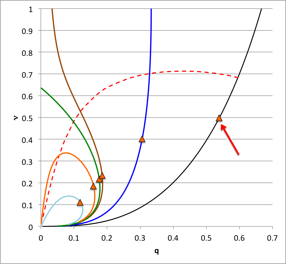
In an accompanying discussion we have shown that we can integrate the linear adiabatic wave equation (LAWE) — that is, we effectively have been able to solve the eigenvalue problem — to obtain the eigenvector associated with marginally unstable models along equilibrium sequences for bipolytropes having <math>~(n_c, n_e) = (5, 1)</math>. The marginally unstable models that have been identified via this more rigorous approach fall at different points along each equilibrium sequence — see the orange triangles in the following figure — than the points that were identified via our free-energy analysis — see the red-dashed demarcation curve. Assuming that the algorithm that we developed to integrate the LAWE was basically error-free, we trust the model identifications generated via this more rigorous technique.

Initial Model Parameters for LAWE-Determined Marginally Unstable Model
<math>~\frac{\mu_e}{\mu_c}</math>	<math>~\xi_i</math>	<math>~\frac{s}{\Re/\bar{\mu}}\biggr\|_\mathrm{core}</math>	<math>~\frac{s}{\Re/\bar{\mu}}\biggr\|_\mathrm{env}</math>
1	1.6686460157	8.04719	1.31310

For more details, see the accompanying discussion titled, Eigenvectors from Solution of LAWE

User:Tohline/Appendix/Ramblings/PatrickMotl

Contents