User:Tohline/Appendix/Ramblings/PatrickMotl
Discussing Patrick Motl's 2019 - 2020 Simulations

|
|---|
| | Tiled Menu | Tables of Content | Banner Video | Tohline Home Page | |
May 1 (from Patrick)
|
Hi Joel, I hope things are well for you and yours. I did finally have a couple research students this semester that were able to slog their way into unix, programming, etc. far enough to do some useful things. They ran two spherical bipolytropes with my old cylindrical code. These were n = 5 cores with n = 1 envelopes. No density discontinuity. One model is a little below the stability boundary in xi, the other is a little above the stability boundary. What I can see from the evolutions, especially now that I made plots of the entropy, is that they are convectively unstable and that is just a mess with the core convecting into the envelope. Did you happen to have any thoughts on what might be a better case to run? When I get done grading finals I am going to work through the equations with kappa set explicitly in the envelope so the entropy profile is flat and just live with whatever density discontinuity that gives me. cheers, Patrick |
May 4 (from Joel)
|
Patrick, My initial response to your 1 May email follows. In an effort to make sure we are on the same page when referencing the structural properties and the stability properties of various configurations, my response includes links to various chapters/subsections of my online wiki-based book. Thanks for pursuing this problem. I am still very interested in Its solution. All the best, Joel |
Chosen Initial Models
I presume that when you constructed your pair of initial (spherical) models, you used the analytically prescribed properties found in my chapter titled, "BiPolytrope with <math>n_c = 5</math> and <math>n_e=1</math>" and that when you reference the "stability boundary in <math>~\xi</math>" you are drawing from the summary (Table 3 and Figure 3) found near the end of this chapter in the subsection titled, "Stability Condition." In particular, based on the information contained in this chapter, I presume that you are assuming that the marginally unstable model along the <math>~\mu_e/\mu_c = 1</math> sequence is the configuration having the properties …
<math>~(\xi_i, q, \nu) = (2.416, 0.5952, 0.6830) \, ,</math>
and that your pair of initial models have values of <math>~\xi_i</math> that are somewhat greater than and somewhat smaller than 2.416. If this does not properly describe your choice of initial models, please clarify.
Instability Toward Convection
In my chapter titled, "Axisymmetric Instabilities to Avoid," I discuss — among other things — the Schwarzschild Criterion. Toward the very end of that chapter, in a subsection titled, Modeling Implications and Advice, I specifically describe how convection might arise when modeling spherical polytropic configurations. Would you please read this short subsection and let me know whether you agree with my explanation or not?
In the context of this discussion of the Schwarzschild criterion (i.e., convective instabilities) in polytropes, my question to you is: What value of the adiabatic index, <math>~\gamma</math>, did you use when you evolved the bipolytrope? Did you use the same index for the entire configuration, or did you use a value in the envelope that is different from the value used in the core?
If you used <math>~\gamma = 6/5</math> for the core, then the core should have uniform specific entropy and therefore would be (only) marginally stable against convection. Likewise, if you used <math>~\gamma = 2</math> for the envelope, it should be (only) marginally stable against convection. Incidentally, these are the two separate values of the adiabatic index that I used when I used a free-energy analysis to examine stability.
NOTE: In yet another chapter of my book, I discuss the bipolytropic stability analysis that was performed by Murphy & Fiedler (1985b). They examined the stability of bipolytropes having the core/envelope polytropic indexes swapped, that is, their equilibrium models had, <math>~(n_c, n_e) = (1, 5)</math>. Their stability analysis was performed while assuming that the adiabatic index was <math>~\gamma = 5/3</math> throughout the entire configuration. In a short subsection near the beginning of my chapter titled, "Aside Regarding Convectively Unstable Core," I have pointed out that the cores of these models should have all been convectively unstable, according to the Schwarzschild criterion. Please read this short subsection and let me know if you agree with my stated expectation for those models.
Other Approaches to Stability Analysis
After you send me feedback on the comments & questions I have presented, above, I have a good deal more to tell you about my analysis of the stability of our <math>~(n_c, n_e) = (5, 1)</math> bipolytropic configurations. I am still a bit confused, but I'm pretty sure that the transition from stable to unstable configurations along the <math>~\mu_e/\mu_c = 1</math> occurs at a value of <math>~\xi_i \approx 1.67</math>, rather than the value of <math>~\xi_i = 2.416</math> that I obtained via the free-energy analysis. But, as I've said, there is a lot to tell you about this.
Other Suggestions
You asked what alternative models might be examined. It might be smarter to first evolve some simpler models, such as pressure-truncated polytropes — not bipolytropes. But we should discuss this after I read your feedback on the above.
May 4 (from Patrick)
May 5 (following a phone conversation with Patrick)
Tying Expressions into H_Book Context
In our wiki-based chapter titled, "First Law of Thermodynamics," we have introduced the concept of an entropy tracer, <math>~\tau</math>. In the subsubsection of this chapter that is titled, "Substantiation," we show that an expression for the specific entropy of a fluid element is,
<math>~s = c_P \ln\biggl( \frac{\tau}{\rho} \biggr) + \mathrm{constant} \, .</math>
In addition, from our wiki-based chapter titled, "Ideal Gas Equation of State," we find the relations,
|
<math>~c_P - c_V </math> |
<math>~=</math> |
<math>~\frac{\Re}{\bar\mu} </math> |
and, |
<math>~\gamma_g </math> |
<math>~=</math> |
<math>~\frac{c_P}{c_V} </math> |
<math>~\Rightarrow</math> |
<math>~c_P </math> |
<math>~=</math> |
<math>~\frac{\gamma_g}{(\gamma_g-1)} \biggl( \frac{\Re}{\bar\mu} \biggr) \, .</math> |
Hence this expression for the entropy may be rewritten as,
<math>~s = \frac{\gamma_g}{\gamma_g-1} \biggl( \frac{\Re}{\bar\mu} \biggr) \ln\biggl( \frac{\tau}{\rho} \biggr) + \mathrm{constant} \, .</math>
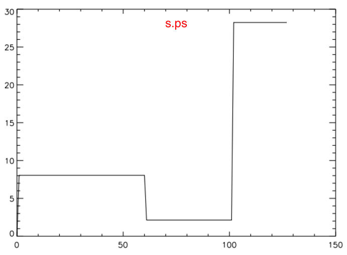
Aside from the factor of <math>~({\bar\mu})^{-1}</math> that appears on the RHS — more on this below — these are the expressions that Patrick has used to generate the s.ps plot, where the (unlabeled) ordinate is the normalized specific entropy, <math>~s/\Re</math>.
At the end of another subsubsection titled, "Initial Recognition," we also find a relevant expression, namely,
<math>~\tau \equiv (\rho\epsilon)^{1/\gamma_g} = \biggl[ \frac{P}{(\gamma_g - 1)} \biggr]^{1/\gamma_g} \, .</math>
Hence, ignoring the additive constant, in general we may write,
|
<math>~\frac{s}{\Re/\bar{\mu}}</math> |
<math>~=</math> |
<math>~ \frac{1}{(\gamma_g-1)}\ln \biggl(\frac{\tau}{\rho}\biggr)^{\gamma_g} </math> |
|
|
<math>~=</math> |
<math>~ \frac{1}{(\gamma_g-1)}\ln \biggl[ \frac{P}{(\gamma_g-1)\rho^{\gamma_g}} \biggr] \, . </math> |
Understanding the Step Function at the Core-Envelope Interface
Now, turning to the accompanying tabular summary of the Radial Profile of Various Physical Variables, we are able to determine how the specific entropy behaves throughout the core and, separately, throughout the envelope in <math>~(n_c, n_e) = (5, 1)</math> bipolytropes.
|
CORE: Throughout the core, we see that,
Hence, independent of the radial location, <math>~\xi</math>, throughout the core,
ENVELOPE: Throughout the envelope, we see that,
Hence, independent of the radial location, <math>~\eta</math>, throughout the envelope,
|
It is therefore clear that the core is a uniform specific-entropy sphere and the envelope is a uniform specific-entropy spherical shell, but in general the specific entropy of material in the envelope is different from the specific entropy of material in the core.
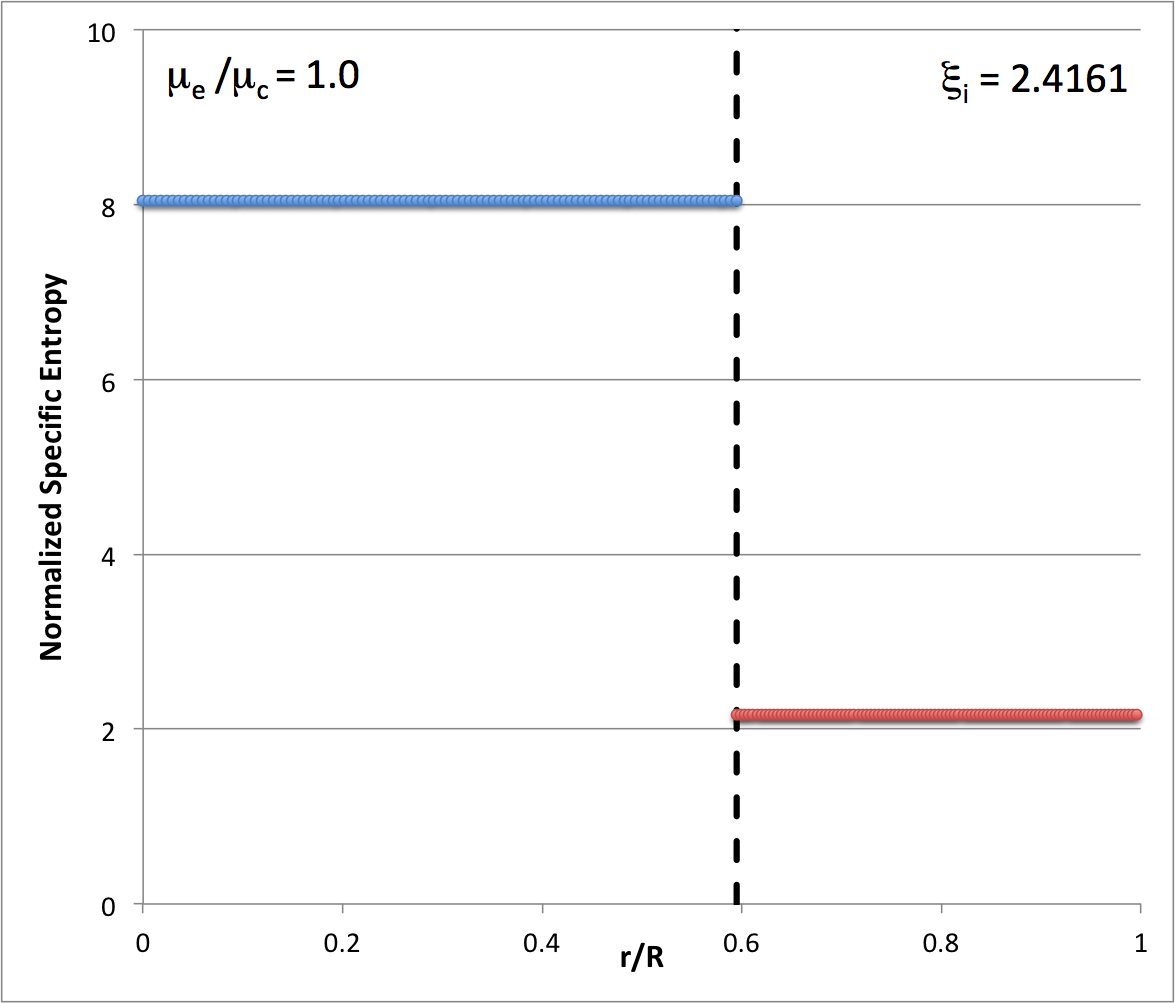
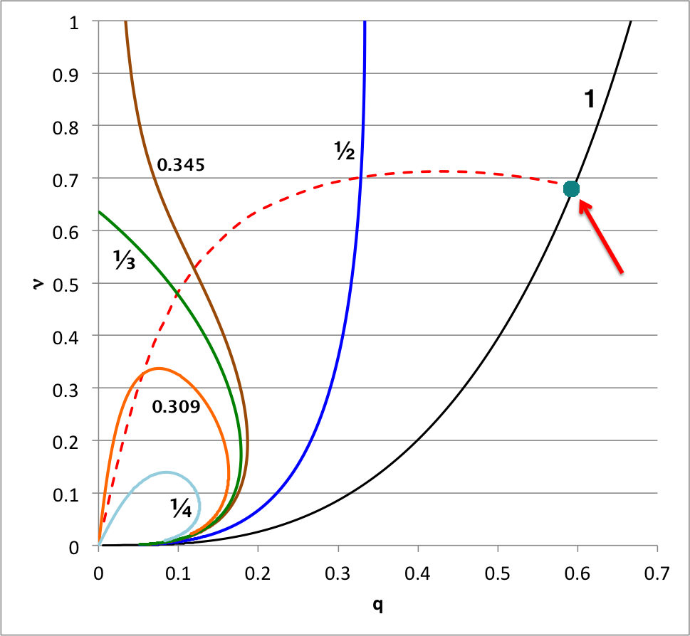
According to our free-energy based evaluation of the stability of bipolytropes having <math>~(n_c, n_e) = (5, 1)</math>, the marginally unstable model along the <math>~\mu_e/\mu_c = 1</math> sequence has the following properties: <math>~(\xi_i, q, \nu, \rho_c/\bar\rho) = (2.41610822, 0.59520261, 0.68306067, 16.3788)</math>; the red arrow in the following diagram points to this model's position in the <math>~q-\nu</math> parameter plane. In an effort to test whether or not this model does identify the transition from stable to unstable configurations along the <math>~\mu_e/\mu_c = 1</math> sequence, Patrick picked a pair of models (highlighted in green in the following table) that straddle the location of the marginally unstable model, and followed the dynamical evolution of both models using a fully 3-D hydrodynamics code. In particular, for the pair of models that Patrick evolved, we find:
| ||||||||||||||||||||||||||||||||||
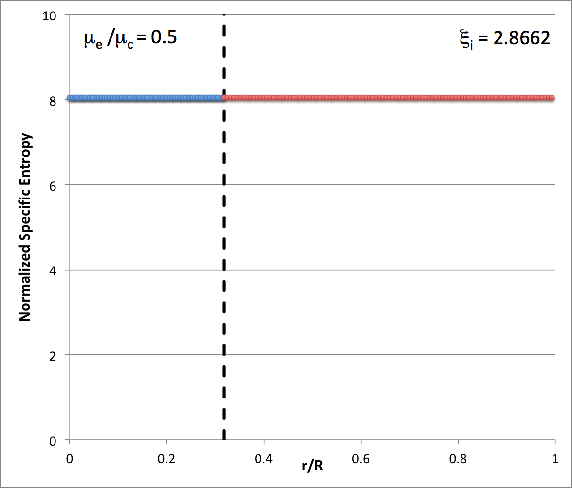
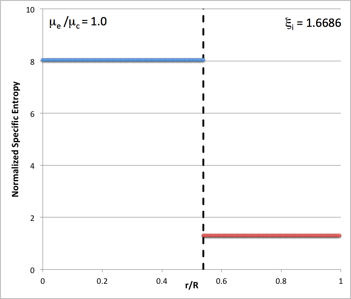
These tabulated values of the normalized specific entropy in the core and, separately, in the envelope — also see the plot shown here on the right — appear to be consistent with Patrick's s.ps plot of specific entropy. In particular, this confirms that a step function should appear at the core-envelope interface and that the specific entropy of the envelope material should be lower than the specific entropy of the core material. Therefore, the Schwarzschild criterion is violated at the interface and we should not have been surprised to see convective motions develop — initially, only at the interface.
Can the Step Function be Flipped or Erased
Assume a Mean-Molecular-Weight Ratio of Unity
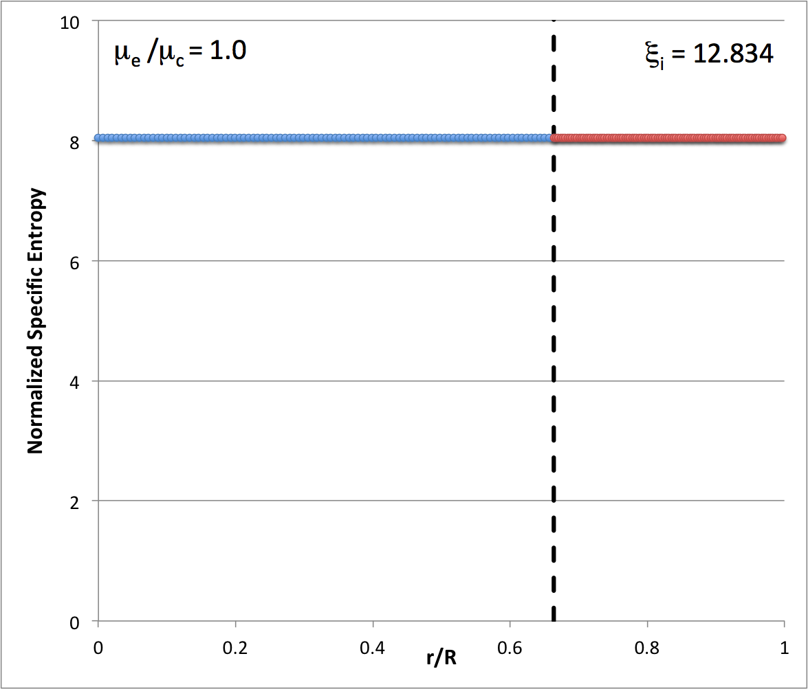
If we continue to examine equilibrium models that have <math>~\mu_e/\mu_c = 1</math>, is there a value of the interface radius, <math>~\xi_i</math>, for which the entropy step-function disappears and above which the step function flips? The answer appears to be, "Yes." It occurs along the equilibrium sequence where the normalized specific entropy has the same value in the core and as in the envelope. That is, it occurs when,
Prediction: Any initial model with <math>~\mu_e/\mu_c = 1</math> and <math>~\xi_i > [\xi_i]_\mathrm{smooth}</math> will be stable against convection, but will be globally dynamically unstable.
Pick a Different Molecular-Weight Ratio
Caution: This subsection contains a derivation that is based on an interpretation of the specific entropy normalization at the interface that may not be physically correct. It needs more thought … After more thought: In order to determine whether the entropy of the envelope is greater than the entropy of the core it would be wise to always plot the specific entropy relative to <math>~\mu_c</math>; therefore, when the ratio <math>~(\tau/\rho)^{\gamma_g}</math> is used to calculate the envelope entropy, <math>~[s/(\Re/\bar\mu)]_\mathrm{env}</math>, as above, the calculated answer should then be divided by <math>~(\mu_e/\mu_c)</math> in order to obtain the proper normalization.
In principle, we can determine in a similar fashion the values of <math>~[\xi_i]_\mathrm{smooth}</math> that are relevant to equilibrium model sequences having <math>~\mu_e/\mu_c < 1</math>. But in doing this, we must take into account that in most of our above derivations the mean-molecular-weight appears in the denominator of the (LHS) expression for the normalized specific entropy. More generally, the prescription for <math>~[\xi_i]_\mathrm{smooth}</math> should come from the demand that,
|
<math>~0</math> |
<math>~=</math> |
<math>~\frac{s_\mathrm{env}}{\Re} - \frac{s_\mathrm{core}}{\Re}</math> |
|
<math>~\Rightarrow ~~~ 0</math> |
<math>~=</math> |
<math>~\frac{1}{\mu_c} \biggl\{\biggl( \frac{\mu_c}{\mu_e} \biggr) \ln \biggl[ \biggl(\frac{\mu_e}{\mu_c}\biggr)^{-2} \biggl( 1 + \frac{\xi_i^2}{3}\biggr)^2 \biggr]_\mathrm{smooth} - 5 \ln(5) \biggr\}</math> |
|
<math>~\Rightarrow ~~~ \ln \biggl[ \biggl(\frac{\mu_e}{\mu_c}\biggr)^{-2} \biggl( 1 + \frac{\xi_i^2}{3}\biggr)^2 \biggr]_\mathrm{smooth} </math> |
<math>~=</math> |
<math>~ \ln\biggl[ 5 \biggr]^{5(\mu_e/\mu_c)} </math> |
|
<math>~\Rightarrow ~~~ \biggl( 1 + \frac{\xi_i^2}{3}\biggr)_\mathrm{smooth} </math> |
<math>~=</math> |
<math>~ 5^{2.5(\mu_e/\mu_c)} \biggl(\frac{\mu_e}{\mu_c}\biggr) </math> |
|
<math>~\Rightarrow ~~~ [\xi_i]_\mathrm{smooth} </math> |
<math>~=</math> |
<math>~ 3^{1 / 2}\biggl[ 5^{2.5(\mu_e/\mu_c)} \biggl(\frac{\mu_e}{\mu_c}\biggr) -1\biggr]^{1 / 2} \, .</math> |
Here are a few examples:
|
Use the Same Ratio of Specific Heats Throughout
Let's examine the initial model's entropy profile under the assumption that the system is evolved with <math>~\gamma_g = 5/3</math> throughout the bipolytrope. From the above analysis, in this case the relevant general expression for the specific entropy profile should be,
|
<math>~\frac{s}{\Re/\bar{\mu}}</math> |
<math>~=</math> |
<math>~ \frac{3}{2} \ln \biggl[ \frac{3P}{2\rho^{5/3}} \biggr] </math> |
<math>~=</math> |
<math>~ \ln \biggl[ \biggl(\frac{3P}{2}\biggr)^{3 / 2} \rho^{-5/2} \biggr] \, . </math> |
|
CORE: Given that, throughout the core,
we have,
ENVELOPE: Given that, throughout the envelope,
we have,
|
| Figure 5 |
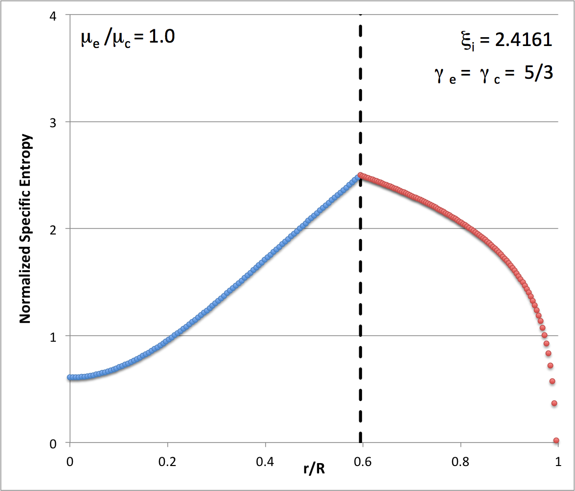 |
Notice that, because <math>~[\gamma_c = 5/3] > [(n_c + 1)/n_c = 6/5]</math>, the specific entropy increases with radius throughout the core, so according to the Schwarzschild criterion the core is stable against convection. However, because <math>~[\gamma_e = 5/3] < [(n_e + 1)/n_e = 2]</math>, the specific entropy decreases with radius throughout the envelope, so according to the Schwarzschild criterion the envelope must be unstable toward convection.
Note: Murphy & Fiedler (1985b) have examined radial oscillation modes in bipolytropic configurations that have a flipped set of indexes — that is, they studied equilibrium structures having <math>~(n_c, n_e) = (1, 5)</math> — assuming, as we have examined here, that oscillations in both the core and the envelope are governed by <math>~\gamma_g = 5/3</math>. The chapter of this H_Book in which we discuss the detailed analysis presented by Murphy & Fiedler, we have inserted a short subsection titled, Aside Regarding Convectively Unstable Core, where we point out that the cores of the Murphy & Fiedler models should be convectively unstable whereas their envelopes should be stable against convection.
Eigenvectors of Marginally Unstable Models
In preparation for our examination of the relative stability of bipolytropic structures having <math>~(n_c, n_e) = (5, 1)</math> — via numerical integration of the Linear-Adiabatic Wave Equation (LAWE) — we have demonstrated that we understand technically how to solve this type of eigenvalue problem by quantitatively reproducing related analyses that have been previously published by other groups.
Good Comparisons With Previously Published Studies
-
Schwarzschild (1941) 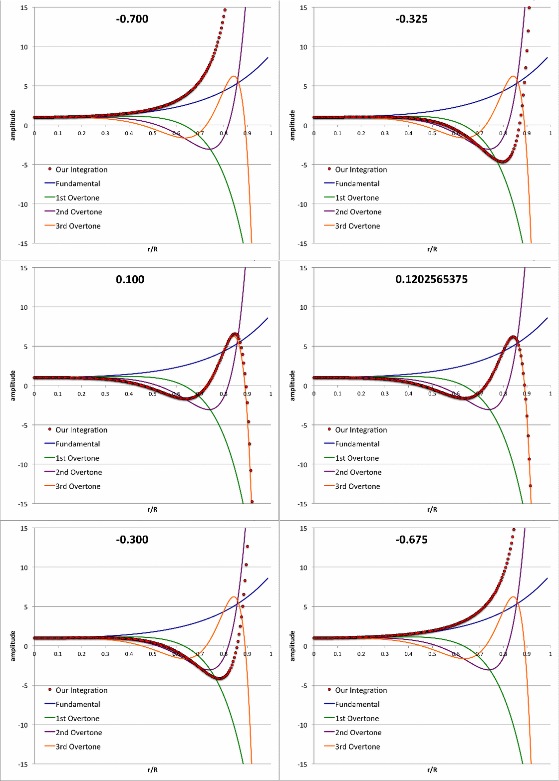
Taff & Van Horn (1974) 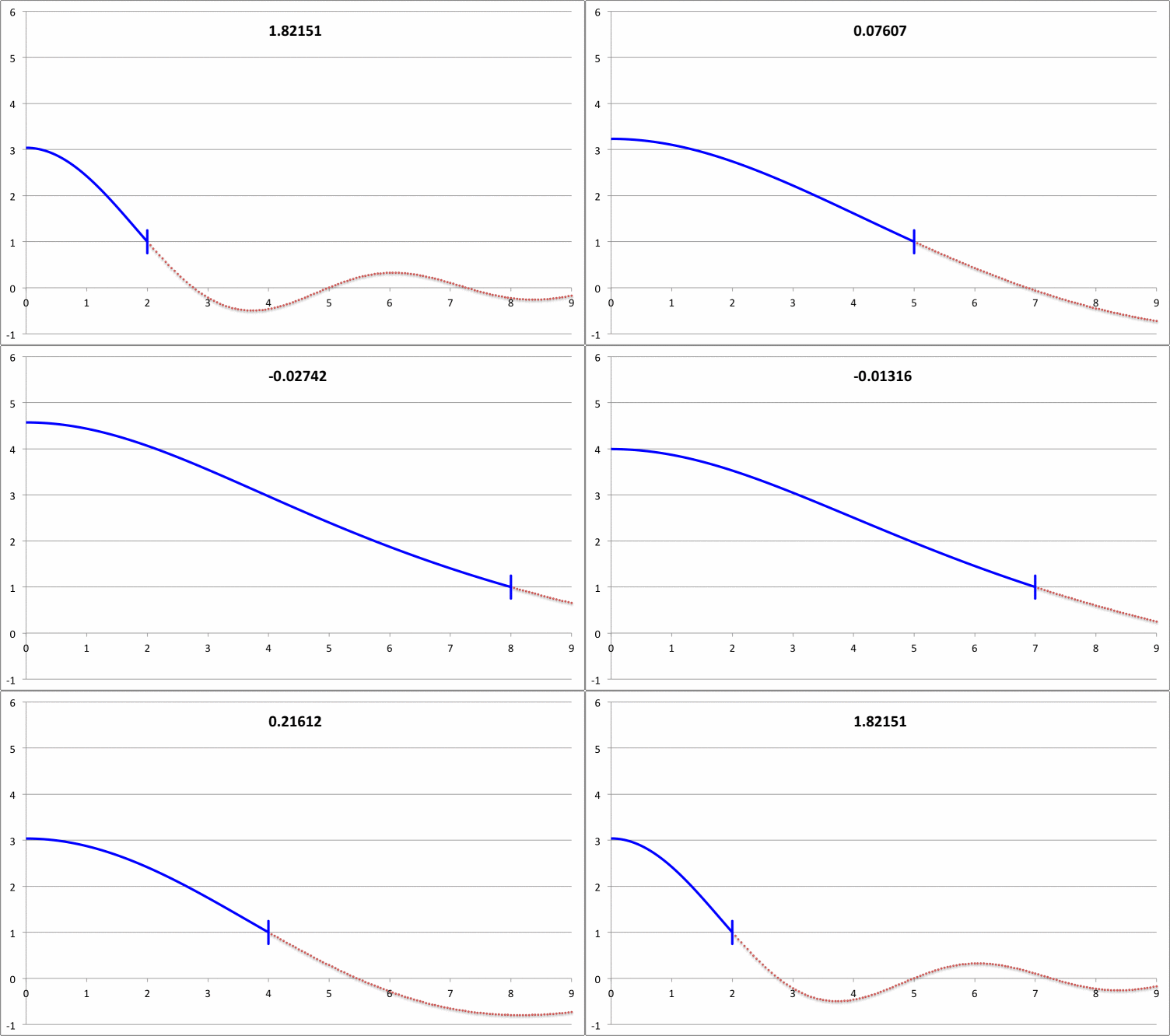
Murphy & Fiedler (1985b) 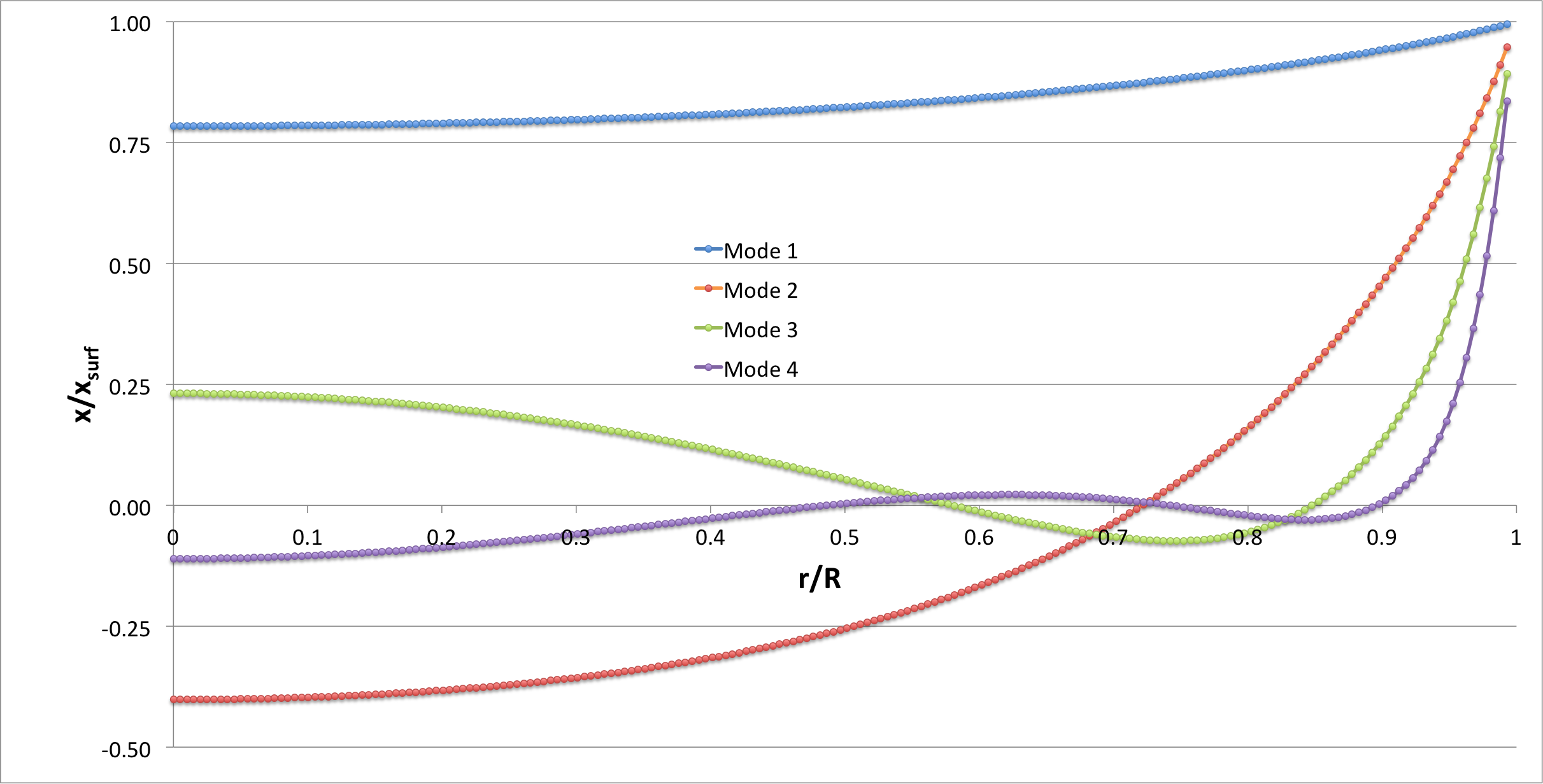
Schwarzschild (1941) numerically integrated the LAWE for isolated <math>~n=3</math> polytropic spheres to find eigenvectors (i.e., the spatially discrete eigenfunction and corresponding eigenfrequency) for five separate oscillation modes (the fundamental mode, plus the 1st, 2nd, 3rd, and 4th overtones) for models having four different adopted adiabatic indexes <math>~\gamma_g = \tfrac{4}{3}, \tfrac{10}{7}, \tfrac{20}{13}, \tfrac{5}{3})</math>. In an accompanying chapter of this H_Book, we demonstrate that we have been able to reproduce in detail Schwarzschild's results for the specific case of <math>~\gamma_g = \tfrac{20}{13}</math>.
- Taff & Van Horn (1974) examined radial oscillations in pressure-truncated isothermal spheres, assuming that the configurations remain isothermal during the oscillations. For models having nine different truncation radii — chosen to straddle the position along the equilibrium sequence where the marginally unstable model was expected to arise — they determined and published the fundamental-mode eigenvalues. For three of these models they also determined and published eigenvalues for the first harmonic mode of oscillation; the radial eigenfunctions associated with both the fundamental mode and the first harmonic mode of these three models also has been displayed in their Figure 1. In a separate accompanying discussion, we demonstrate that we have been able to reproduce in detail the subset of eigenfunctions and associated eigenvalues that have been previously published by Taff & Van Horn (1974).
- In their published study of bipolytropes having <math>~(n_c, n_e) = (1,5)</math> with <math>~\mu_e/\mu_c = 1</math>, Murphy & Fiedler (1985b) integrated a coupled pair of LAWEs — one for the core and another for the envelope — to determine the eigenfunctions and corresponding eigenvalues of various radial modes of oscillation in more than a dozen different equilibrium models, assuming that during the oscillations, <math>~\gamma_g = 5/3</math> throughout both the core and the envelope. In an accompanying chapter of this H_Book titled, Review of the BiPolytrope Stability Analysis by Murphy & Fiedler (1985b), we show that we have been able to duplicate in quantitative detail the eigenvectors associated with their equilibrium Models 10 and 17.
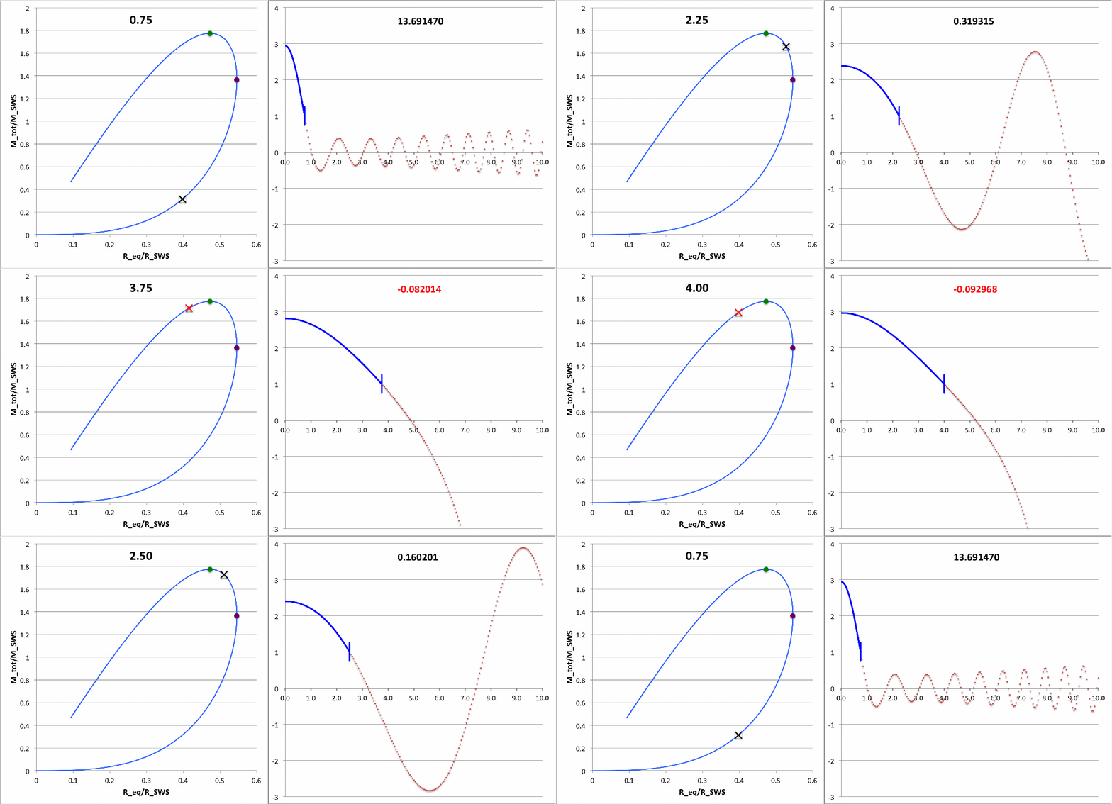
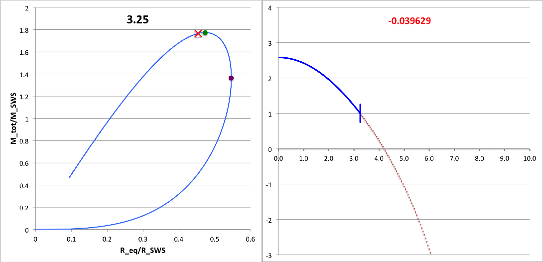
Building upon this set of successful comparisons with stability analyses published by other groups, we have carried out numerical integrations of the relevant LAWE to identify the eigenvectors associated with the fundamental-mode of radial oscillation in pressure-truncated, <math>~n = 5</math> polytropic configurations. Details of this analysis are provided in yet another chapter of this H_Book. The following animation sequence illustrates the results of this analysis. As far as we have been able to determine, an analysis of this type has not previously been conducted for pressure-truncated, <math>~n = 5</math> polytropes.
In a subsection of this separate chapter, we have also shown that, at the maximum-mass turning point along the pressure-truncated <math>~n=5</math> equilibrium sequence — identified by the green circular marker in the left-hand panel of this animation — the fundamental-mode eigenfrequency is precisely zero and the associated eigenfunction is described exactly by the formula for a parabola.
Our Numerical Analysis of Bipolytropes Having (nc, ne) = (5, 1)
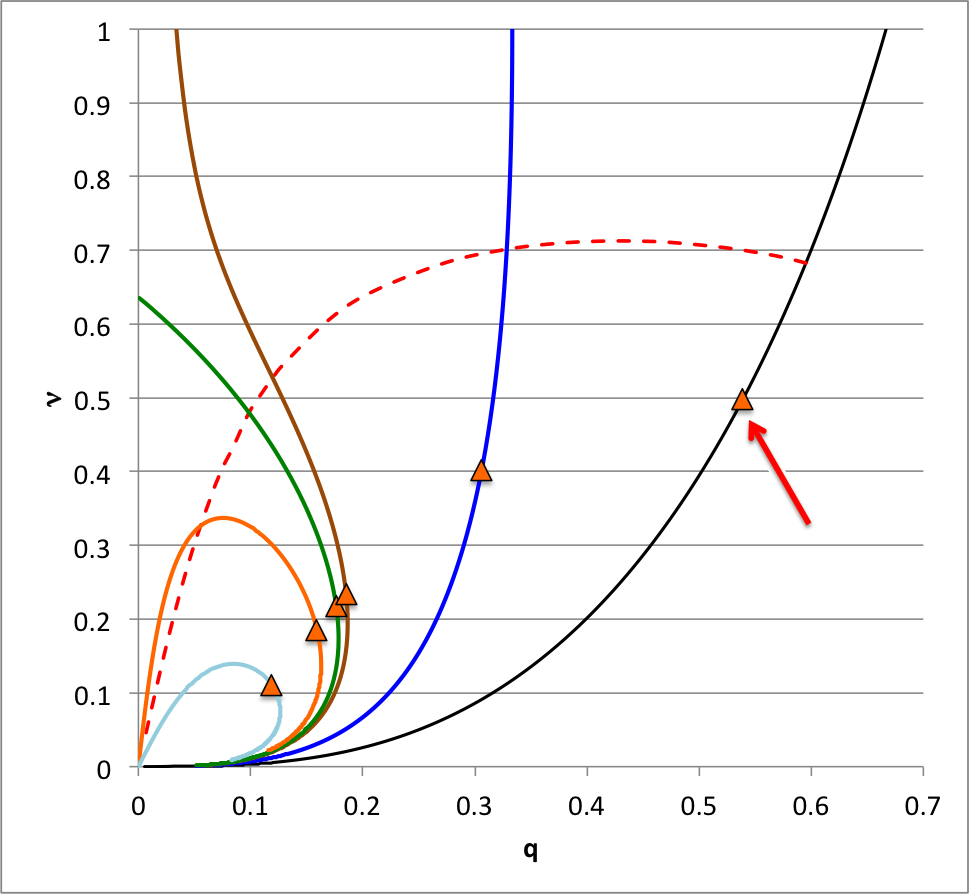
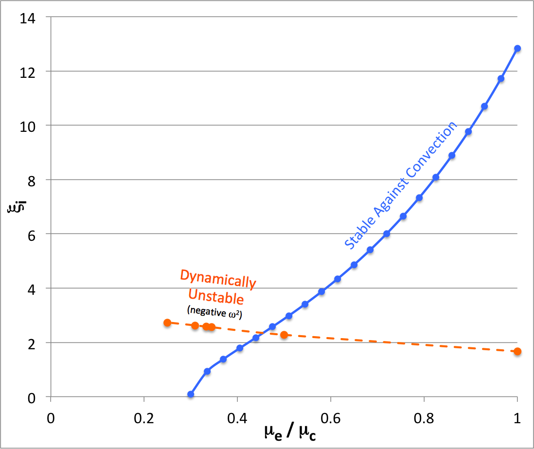
In an accompanying discussion we have shown that we can integrate the linear adiabatic wave equation (LAWE) — that is, we effectively have been able to solve the eigenvalue problem — to obtain the eigenvector associated with marginally unstable models along equilibrium sequences for bipolytropes having <math>~(n_c, n_e) = (5, 1)</math>. The marginally unstable models that have been identified via this more rigorous approach — see the orange triangles in the following figure — fall at different points along each equilibrium sequence than the points that were identified via our free-energy analysis — see the red-dashed demarcation curve. Assuming that the algorithm that we developed to integrate the LAWE was basically error-free, we trust the model identifications generated via this more rigorous technique.
Our analysis indicates that, along the <math>~\mu_e/\mu_c = 1</math> equilibrium sequence, the core-envelope interface of the marginally unstable model is located at <math>~\xi_i = 1.6686460157</math>; in the following figure, the red arrow points to this location along that sequence. In the brief table that accompanies the figure, we have listed values for the dimensionless specific entropy in the core and, separately, in the envelope, along with the interface location, <math>~\xi_i</math>.
| ||||||||||||||||||||||||||
Summary
For three separate equilibrium sequences — specifically, for the cases of <math>~\mu_e/\mu_c = 1, \tfrac{1}{2}, \tfrac{1}{3}</math> — the table on the left, below, identifies the location <math>~(\xi_i)</math> along the sequence where the model is marginally unstable toward a global, dynamical instability as estimated by the our free-energy analysis (column 2) and as determined by our numerical integration of the coupled pair of governing LAWEs (column 6). For each identified model, the corresponding values of <math>~q, \nu</math> and <math>~\rho_c/\bar\rho</math> are also provided. Additional details can be found in our accompanying discussion of, respectively, our free-energy analysis and our numerical solution of the relevant eigenvalue problem.
| |||||||||||||||||||||||||||||||||||||||||||||||||||||||||
In the figure shown here on the right, the orange-dashed curve shows how <math>~\xi_i</math> (table column 6) varies with <math>~\mu_e/\mu_c</math> (table column 1) for marginally unstable models as determined by our numerical eigenvector analysis. The square of the fundamental-mode eigenfrequency is negative for all models above this orange-dashed curve, indicating that they should be globally dynamically unstable. The solid blue curve shows how <math>~[\xi_i]_\mathrm{smooth}</math> varies with <math>~\mu_e/\mu_c</math>, as derived above. Models above and to the left of this blue curve should be stable against convection at the core-envelope interface.
May 11 (from Joel)
|
Patrick, Following our phone conversation earlier this week, I have added a number of paragraphs, derivations, and tables/figures to my VisTrails wiki page — see the above subsection dated, May 5. Here is a quick summary, assuming evolutions are conducted with <math>~(\gamma_c, \gamma_e) = (6/5, 2)</math>:
If you set <math>~\mu_e/\mu_c = 1</math> but assume evolutions are conducted with <math>~\gamma_c = \gamma_e = 5/3</math>:
Finally, we should consider the following before embarking on more 3D simulations:
Other things to discuss:
I am very interested in discussing all of this with you, if you are interested and when you have the time. Just let me know. Cheers, Joel |
May 14 (from Patrick)
|
Hi Joel, There are some movies and plots on line at http://patrickmotl.net if you follow the links for bipolytropic stars with n_core = 5 and n_envelope = 1 |
Patrick and Joel also had a long phone conversation on this date, 14 May 2019.
Discussing Simulations of Pressure-Truncated n = 5 Polytropes
September 22, 2020 (from Patrick)
|
Hi Joel I am going to talk (by zoom) for a little bit next Tuesday [i.e., on 29 September 2020] on the n = 5 polytropes my students ran in the spring and summer for the LSU astro lunchtime seminar. Very short version is that when truncated at xi < 3 they oscillate. At larger radii, they all collapsed. I am attaching the abstract for the talk for the longer version. Anyway, I was hoping that saying yes to Manos for a speaking slot would force me to analyze data, make movies, etc. It would be great if you popped in on the seminar. If that doesn’t work, it would also be great to chat in zoom at some other time. |
October 06
In preparation for this afternoon's Zoom session (between just Patrick and Joel), Joel should look at plots and movies under the category, "Joshue's pressure truncated n = 5 polytropes," found on Patrick's primary web site.
During the Zoom session, the question arose whether or not there was a straightforward way for Patrick (and his students) to compare their measured oscillation frequencies and measured eigenfunctions with predictions of LAWE.
October 07 - 08 (between Joel & Patrick)
|
Patrick, Please look at figure 6 and the lines of text that immediately precede and that immediately follow this figure on the following web page: https://www.vistrails.org/index.php/User:Tohline/Appendix/Ramblings/PatrickMotl I put this material together some months ago, but had since forgotten about it. It contains quantitative results that will significantly strengthen any presentation that you make to show the results of your student's 3D simulations. I have carried out a numerical, linear-stability analysis of models along the pressure-truncated, n = 5 model sequence. Specifically, I have numerically determined the eigenfunction and the eigenfrequency (squared) of the fundamental mode of oscillation for 16 different models falling between \xi_i = 0.75 and \xi_i = 5.0. You should plot omega-squared versus \xi_i from this linear-stability analysis, then plot your oscillation frequencies on the same graph to see if they lie along the curve that you get from my analysis. Also, can you actually generate a plot of the radial eigenfunction of the vibration modes that develop in your simulations? You could directly compare these eigenfunction plots against my Figure-6 eigenfunction plots. [I'll be happy to explain this in more detail via a zoom session, if that would help.] Seeing how your results compare to my linear analysis **quantitatively** will be a lot of fun!! We can then march boldly toward a similar analysis of bipolytropes! |
|
Hi Joel, So, measuring the frequencies is relatively straightforward. For the eigenfunction, do you know off the top of your head or a reference for rewriting variation in r over r in terms of variation of rho over rho? I am trying to think of something I can measure from the simulations. |
|
Patrick, This question also popped up in my mind while lying in bed last night. That is, I recognized that the variation in r is a **lagrangian** measurement and you are not set up to make that measurement easily. So you probably need the density variation. I am quite sure that the answer is buried in the following chapter of my on-line book: https://www.vistrails.org/index.php/User:Tohline/SSC/Perturbations#Summary_Set_of_Linearized_Equations For example, this specific link will take you to a subsection of the chapter that gives the relationship between p (fractional pressure variation), d (density), and x (lagrangian radial location) via the three key linearized **differential** equations. I am going to look for a better answer to your question, though. |
October 11
Here's one reasonable way to consider plotting the eigenfunction at various points in time from the nonlinear simulations of oscillating/collapsing, pressure-truncated n = 5 polytropes. (It assumes, even though Patrick's simulation is conducted on a cylindrical-coordinate mesh, that he is able to extract a radially dependent <math>~M_r</math> function from the density data.)
Drawing from an accompanying discussion, we recognize that, in the unperturbed equilibrium state,
|
<math>~m_\xi \equiv \frac{M_r}{M_\mathrm{tot}}</math> |
<math>~=</math> |
<math>~ \biggl(\frac{\xi}{\tilde\xi}\biggr)^3 \biggl(1 + \frac{\xi^2}{3}\biggr)^{-3/2} \biggl(1 + \frac{\tilde\xi^2}{3}\biggr)^{3/2} \, ,</math> |
|
<math>~r_\xi</math> |
<math>~=</math> |
<math>~\xi \biggl\{ \biggl[ \frac{4\pi}{2^5\cdot 3}\biggr]^{1/2} \tilde\xi^{-6} \biggl( 1+\frac{\tilde\xi^2}{3} \biggr)^{3}\biggr\} \, , </math> |
where the "tilde" indicates the value of <math>~\xi</math> at the surface of the pressure-truncated configuration. Usually this parametric relationship between mass and radius is used to generate a plot showing how the mass interior to <math>~r</math> varies with the Lagrangian coordinate, <math>~r</math>, in the equilibrium state. But it can just as well be used to show how <math>~r</math> varies with the Lagrangian coordinate, <math>~m_\xi</math>, in the equilibrium state. Note that these two expressions can be combined to give <math>~r_\xi</math> in the unperturbed configuration — hereafter referred to as <math>~r_0</math> — directly in terms of the fractional mass, <math>~m_\xi</math>; namely,
|
<math>~ r_0 (m_\xi) </math> |
<math>~=</math> |
<math>~\tilde{r}_\mathrm{edge} \biggl[\frac{3^2m_\xi^{2/3}}{\tilde{C} - 3 m_\xi^{2/3}}\biggr]^{1/2} \, , </math> |
where,
|
<math>~\tilde{C}</math> |
<math>~\equiv</math> |
<math>~ \frac{3^2}{\tilde\xi^2}\biggl( 1 + \frac{\tilde\xi^2}{3} \biggr) \, , </math> and, |
|
<math>~\tilde{r}_\mathrm{edge}</math> |
<math>~\equiv</math> |
<math>~\biggl[ \frac{\pi}{2^3\cdot 3}\biggr]^{1/2} {\tilde\xi}^{-6} \biggl(1+\frac{\tilde\xi^2}{3}\biggr)^3 \, . </math> |
TEST: After Patrick introduces a model of given <math>~\tilde\xi</math> into the hydrocode, he should integrate over the density distribution to generate a numerically determined plot of <math>~r</math> versus <math>~m_\xi \equiv M_r/M_\mathrm{tot}</math>, then compare the plot to this analytically specified function for <math>~r_0(m_\xi)</math>. The degree to which the plots match at time, <math>~t = 0</math>, will give a measure of the uncertainty in the numerically determined eigenfunction at later times in the evolution.
At any later time in an evolution, Patrick can again integrate over the density distribution to generate new, numerically determined values of <math>~r(m_\xi)</math>. From this new data, he can generate a plot of the fractional displacement,
|
<math>~x(m_\xi)</math> |
<math>~\equiv</math> |
<math>~\frac{ [r_0(m_\xi) - r(m_\xi) ]}{r_0(m_\xi)} \, .</math> |
Ideally, if oscillations of the model are due entirely to a single radial mode …
- The shape of this fractional displacement function should not change with time; but
- The overall amplitude is expected to vary with time at a frequency that is predicted by linear theory.
Figure 6, above, quantifies the eigenfrequency and the shape of the displacement function for fifteen different models; for the marginally unstable model, the eigenfrequency is zero and the eigenfunction (displacement function) is exactly a parabola.
NOTE: Because the model evolutions are being performed on an Eulerian mesh while the numerically determined quantity, <math>~m_\xi</math>, is a Lagrangian tracer, the array of <math>~m_\xi</math> grid points at which <math>~r</math> is measured will vary with time. This could pose a problem because both of the variables on the right-hand-side of the <math>~x(m_\xi)</math> expression need to be evaluated on the same Lagrangian-tracer grid. Fortunately, we have an analytic expression for <math>~r_0(m_\xi)</math>; so, each time a new Lagrangian-tracer grid arises during the numerical evaluation of <math>~r(m_\xi)</math>, this analytic expression for <math>~r_0(m_\xi)</math> should be called upon to give values of <math>~r_0</math> on the revised Lagrangian-tracer grid. 8
December 22, 2020 (from Patrick)
|
I added several simulations to my web page; these are version 12 of the n = 5 pressure truncated polytropes. I had the code compute the mass profile of the star during the run and plotted Joel’s function x versus enclosed mass as a proxy for the perturbation to the star. I also added plots of the frequency spectrum of the central density perturbation. I plotted the frequency spectrum where time is measured in units of the free fall time. It appears to me that the eigenfrequencies are all evenly spaced which is not what I expected. |
December 30 (Joel's Reply)
Initial Comments
First, I need to make sure that I understand the new plots that you have provided. For discussion purposes, I'll focus on your plots for n = 5 polytrope ξ = 3.25 and constant pressure truncation mark 12. It appears to me that a key plot/animation is the "x versus m" plot shown in the upper-right corner of this web page; on your web page this plot/animation is labeled, "<math>~(R - R_0)/R_0</math> vs Mass." I presume that this shows the time-evolution of the radial eigenfunction; am I correct? Immediately below, I have reproduced one frame from this movie.
|
Above: A frame showing radial eigenfunction from Motl's nonlinear simulation of model having initial <math>~\tilde\xi = 3.25</math>. Below-right: A frame from the Tohline's "Composite Display 1," showing eigenfunction from Tohline's solution of the LAWE for the same initial model. |
We expect Motl's eigenfunction to lie right on top of the blue segment of Tohline's eigenfunction. The good news is that, at least at first glance, the two eigenfunctions look quite similar. But we need to generate new plots having the same axes. For example, Tohline's eigenfunction plot is x versus R0 whereas Motl's plot shows x versus m. Note that the vertical amplitude (x) can be rescaled to an arbitrary value at the center.
What about the eigenfrequency? Well, for the model with an initial value of <math>~\tilde\xi = 3.25</math>, Tohline's solution of the LAWE gives <math>~\sigma_c^2 = - 0.039629</math>. What value is obtained from Motl's simulation? Well … I don't quite know how to interpret Motl's plot of <math>~|F(\rho)|</math> versus <math>~f/f_0</math>. But Motl's plot of <math>~\rho</math> versus <math>~t/T_0</math> ought to tell us something. Because <math>~\sigma_c^2</math> is negative, this model is dynamically unstable and it should collapse on the timescale of a single oscillation frequency <math>~\sigma_c = \sqrt{0.039629} \approx 0.200</math>. If Motl generates a semi-log plot — that is <math>~\ln\rho</math> versus <math>~t/T_0</math>, he should see a line with slope given by this value of <math>~\sigma_c</math>. NOTE: The relationship between <math>~\sigma_c</math> and <math>~\omega</math> is given in the following subsection.
Material that appears after this point in our presentation is under development and therefore
may contain incorrect mathematical equations and/or physical misinterpretations.
| Go Home |
Additional Information on Frequencies
In our accompanying derivation of the LAWE, we define the perturbations in pressure ( p ), density ( d ), and Lagrangian radial position ( x ) such that,
|
<math>~P(m,t)</math> |
<math>~=</math> |
<math>~P_0(m) + P_1(m,t) = P_0(m) \biggl[1 + p(m) e^{i\omega t} \biggr] \, ,</math> |
|
<math>~\rho(m,t)</math> |
<math>~=</math> |
<math>~\rho_0(m) + \rho_1(m,t) = \rho_0(m) \biggl[1 + d(m) e^{i\omega t} \biggr] \, ,</math> |
|
<math>~r(m,t)</math> |
<math>~=</math> |
<math>~r_0(m) + r_1(m,t) = r_0(m) \biggl[1 + x(m) e^{i\omega t} \biggr] \, .</math> |
Let's focus on the time-dependent behavior of the central density. Whenever <math>~\omega^2</math> is negative, we appreciate that <math>~\omega</math> will be imaginary so the exponent of the exponential will be real. In this case, we expect the central density to grow exponentially (cloud collapse); its behavior will be described by the expression,
|
<math>~\frac{\rho(t)}{\rho_0} \biggr|_c</math> |
<math>~=</math> |
<math>~ 1 + d_c e^{\sqrt{\omega^2}t} \, . </math> |
(Note: In what follows, we will assume for simplicity that the radial eigenfunction for the perturbed density, <math>~d(m)</math>, is normalized such that it is unity at the center (i.e., at m = 0); that is, we will set <math>~d_c = 1</math>.)
Now, the frequency, <math>~\omega</math>, has units of inverse time. Also, in the chapter where we specifically study pressure-truncated n = 5 ploytropes, we define the dimensionless frequency,
|
<math>~\sigma_c^2</math> |
<math>~\equiv</math> |
<math>~\frac{3\omega^2}{2\pi G \rho_c} \, .</math> |
Realizing that, in Patrick's plots,
<math>~T_0 \equiv \biggl[\frac{3\pi}{32 G \bar\rho}\biggr]^{1 / 2} \, ,</math>
where,
|
<math>~\bar\rho</math> |
<math>~\equiv</math> |
<math>~\frac{3M_\mathrm{tot}}{4\pi R_\mathrm{eq}^3} \, ,</math> |
we see that the exponent in the exponential may be rewritten as,
|
<math>~\sqrt{\omega^2} t</math> |
<math>~=</math> |
<math>~ \sqrt{\sigma_c^2} \biggl(\frac{2\pi G \rho_c}{3}\biggr)^{1 / 2} \biggr(\frac{t}{T_0}\biggr) \biggl[\frac{3\pi}{32 G \bar\rho}\biggr]^{1 / 2} </math> |
|
|
<math>~=</math> |
<math>~ \sqrt{\sigma_c^2} \biggr(\frac{t}{T_0}\biggr) \frac{\pi}{4}\biggl[\frac{\rho_c}{\bar\rho}\biggr]^{1 / 2} </math> |
Now, from our accompanying discussion of the integration form factors for truncated n = 5 polytopes, we know that,
|
<math>~\mathfrak{f}_M \biggr|_{n=5}</math> |
<math>~=</math> |
<math>~ \frac{\bar\rho}{\rho_c} \biggr|_{n=5} = \biggl[ 1 + \frac{{\tilde\xi}^2}{3} \biggr]^{-3 / 2} \, . </math> |
| Selected Models | |||||
| <math>~\tilde\xi</math> | <math>~\frac{M_\mathrm{tot}}{M_\mathrm{SWS}}</math> | <math>~\frac{R_\mathrm{eq}}{R_\mathrm{SWS}}</math> | <math>~\frac{\rho_c}{\bar\rho}</math> | <math>~\sigma_c^2</math> | <math>~\sqrt{\omega^2} t</math> |
| 2.75 | - | - | 6.6065 | +0.061925 | 0.50235 <math>~\biggl(\frac{t}{T_0} \biggr)</math> |
| 3 | 1.77408 | 0.47309 | 8 | 0.0 | 0.0 <math>~\biggl(\frac{t}{T_0} \biggr)</math> |
| 3.25 | - | - | 9.6123 | - 0.039629 | 0.48474 <math>~\biggl(\frac{t}{T_0} \biggr)</math> |
| 3.5 | - | - | 11.4610 | - 0.065282 | 0.67936 <math>~\biggl(\frac{t}{T_0} \biggr)</math> |
As we have detailed in a separate discussion, for pressure-truncated n = 5 polytropes,
|
<math> \frac{M_\mathrm{tot}}{M_\mathrm{SWS}} </math> |
<math>~=~</math> |
<math> \biggr( \frac{3^{2} \cdot 5^3 }{4\pi } \biggr)^{1/2} \frac{\tilde\xi^{3}}{(3 + \tilde\xi^2)^{2}} \, , </math> |
|
<math> \frac{R_\mathrm{eq}}{R_\mathrm{SWS}} </math> |
<math>~=~</math> |
<math> \biggr( \frac{3^{2} \cdot 5}{2^2 \pi } \biggr)^{1/2} \frac{\tilde\xi}{(3 + \tilde\xi^2)} \, . </math> |
December 31, 2020 (from Patrick)
|
I am attaching plots of density for xi = 3.5, 3.25. The dashed lines are for exp(sigma_c t) where t is measured in free fall times and I took sigma from your animated gif. 0.19907 for xi of 3.25 and 0.25550 for xi of 3.5. I don’t think it is the growth of just one mode. |
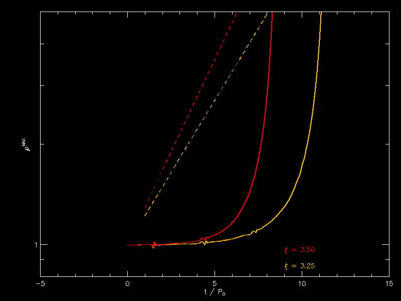 |
Joel's interpretation: Measuring the slopes of the dashed lines directly from the figure, I obtain the following slopes. First, the starting and ending points of the red dashed-line segment appear to be, respectively, <math>~(\rho_c, t/P_0) = (1.00, 0.00)</math> and <math>~(\rho_c, t/P_0) = (5.00, 6.25)</math>. Hence …
| For <math>~\tilde\xi = 3.5~</math>: |
<math>~\frac{\Delta \ln\rho_c}{\Delta t/P_0}</math> |
<math>~=</math> |
<math>~ \frac{\ln(5.0) - \ln(1.0)}{6.25 - 0} = \frac{1.6094}{6.25} = 0.2575 \, . </math> |
This is consistent with <math>~\sigma_c = \sqrt{0.065282} = 0.25555</math>, which is the value that I said comes from the linear-stability analysis. Second, the starting and ending points of the yellow dashed-line segment appear to be, respectively, <math>~(\rho_c, t/P_0) = (1.00, 0.00)</math> and <math>~(\rho_c, t/P_0) = (5.00, 8.05)</math>. Hence …
| For <math>~\tilde\xi = 3.25~</math>: |
<math>~\frac{\Delta \ln\rho_c}{\Delta t/P_0}</math> |
<math>~=</math> |
<math>~ \frac{\ln(5.0) - \ln(1.0)}{8.05 - 0} = \frac{1.6094}{8.05} = 0.1999 \, . </math> |
This is consistent with <math>~\sigma_c = \sqrt{0.039629} = 0.1991</math>, which is the value that I said comes from the linear-stability analysis. Okay. I understand Patrick's plot.
January 4, 2021 (Clearer Thoughts from Joel)
Slope in Semi-log Plots
We need to change the way we analyze Patrick's hydro-data output. First, note that Patrick's figure (black background with yellow and red dashed-line segments) is a plot of,
|
<math>~\log_{10}\biggl\{\frac{\rho(t)}{\rho_0}\biggr|_c \biggr\}</math> |
vs. |
<math>~\frac{t}{P_0} \, .</math> |
But, as has been stated in our earlier comments, from the standpoint of a linear-perturbation analysis,
|
<math>~\biggl\{ \frac{\rho(t)}{\rho_0} \biggr|_c \biggr\}</math> |
<math>~=</math> |
<math>~ 1 + d_c e^{\sqrt{\omega^2}t} \, . </math> |
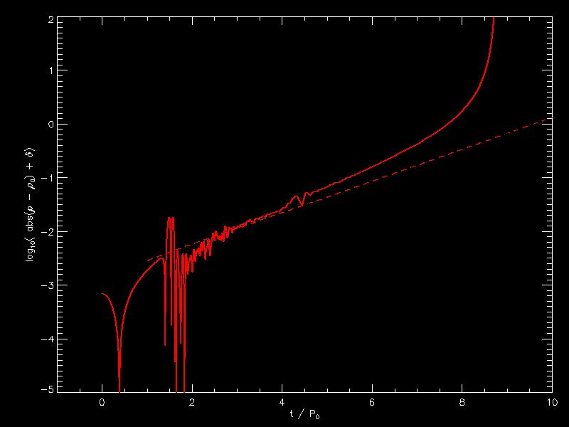
So we should not expect the plots of <math>~\rho_c(t)</math> in Patrick's (black background) figure to show a linear relationship. Instead, we should be plotting the quantity,
|
<math>~\log_{10}\biggl\{\frac{\rho(t)}{\rho_0}\biggr|_c - 1\biggr\}</math> |
vs. |
<math>~\frac{t}{P_0} \, .</math> |
Over the earliest phase of the hydrodynamical simulation while the deviation from the initial model's structure is still quite small — say, for times, <math>0 \le t/P_0 \le 5</math> — such a plot should reveal the following linear relationship:
|
<math>~\log_{10}\biggl\{ \frac{\rho(t)}{\rho_0} \biggr|_c - 1\biggr\}</math> |
<math>~=</math> |
<math>~ \log_{10}(d_c) + \log_{10} \biggl[ e^{\sqrt{\omega^2}t} \biggr] </math> |
|
|
<math>~=</math> |
<math>~ \log_{10}(d_c) + (\log_{10}e) \cdot \ln \biggl[ e^{\sqrt{\omega^2}t} \biggr] </math> |
|
|
<math>~=</math> |
<math>~ \log_{10}(d_c) + 0.434294 \cdot \sqrt{\omega^2}t \, . </math> |
|
Alternatively, we can use natural logarithms throughout, which gives,
|
Converting to <math>~\sigma_c^2</math>, as above, we therefore have,
|
<math>~\log_{10}\biggl\{ \frac{\rho(t)}{\rho_0} \biggr|_c - 1\biggr\}</math> |
<math>~=</math> |
<math>~ \log_{10}(d_c) + 0.434294 \cdot \biggl[\frac{\pi}{4}\biggl( \frac{\rho_c}{\bar\rho}\biggr)^{1 / 2}\biggr] \sqrt{\sigma_c^2} \biggr(\frac{t}{T_0}\biggr) \, . </math> |
Hence,
| For <math>~\tilde\xi = 3.25~</math>: |
<math>~\log_{10}\biggl\{ \frac{\rho(t)}{\rho_0} \biggr|_c - 1\biggr\}</math> |
<math>~=</math> |
<math>~ \log_{10}(d_c) + 0.434294 \cdot \biggl[0.48847\biggr] \biggr(\frac{t}{T_0}\biggr) \, ; </math> and, |
| For <math>~\tilde\xi = 3.5~</math>: |
<math>~\log_{10}\biggl\{ \frac{\rho(t)}{\rho_0} \biggr|_c - 1\biggr\}</math> |
<math>~=</math> |
<math>~ \log_{10}(d_c) + 0.434294 \cdot \biggl[0.67936\biggr] \biggr(\frac{t}{T_0}\biggr) \, . </math> |
NOTE: Even though we know analytically what the (spherically symmetric) expression is for the equilibrium model's radial density distribution, when this model is introduced into the hydrocode's grid, there inevitably will be some noise. In particular, the value of the central density at time <math>~t = 0</math> will not be perfectly correct. The parameter, <math>~d_c</math> — perhaps on the order of 10-2 or 10-6 — represents the amplitude of this departure from the correct value at the start of a hydrodynamic simulation; we won't know its value until the simulation has been completed and this linear function is fit to the plotted data. Alternatively, given that we know from Joel's linear stability analysis what the eigenfunction is for the fundamental mode of oscillation, Patrick could introduce this eigenfunction with a known, specified amplitude into the initial density distribution. But, first, let's see how the "linear fit" works without introducing a particular initial perturbation.
Radial Displacement Function
Our discussion in the previous sub-section has focused on a "linear" stability analysis of the time-dependent behavior of the model's central (maximum) density. Ultimately, I think we would be better off analyzing in an analogous fashion the time-dependent behavior of the radial displacement function. But, first, let's see if an analysis of the central density makes sense.
January 4, 2021 (from Patrick)
|
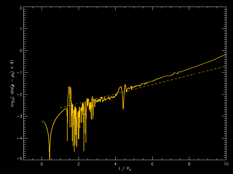
I didn’t play with the offset value too much. 1e-3 seems too small, 2e-3 is too small so I used 1.5e-3 for both in these plots What is plotted on the y axis is the base 10 logarithm of the absolute value of the central density minus 1 (which is the initial density) and then I add 1e-15 to the absolute value to prevent NaN. |
| <math>~\tilde\xi = 3.25</math> | <math>~\tilde\xi = 3.5</math> |
| Log-Amplitude vs. Time for Central-Density Perturbation | |
 |
 |
| Data Used to Plot Radial Displacement Function, <math>~x(\xi)</math>, from Linear-Stability Analysis (see blue segments of Figure 6, above) | |
Eigenvector for pressure-truncated, n = 5 polytrope. \tilde\xi = 3.25 sigma_c^2 = -0.039629467 xi x x(renorm) 0 1 2.58142807 0.05 0.999843241 2.581023407 0.1 0.999372999 2.579809512 0.15 0.998589419 2.577786756 0.2 0.997492732 2.574955737 0.25 0.99608326 2.571317288 0.3 0.994361421 2.566872483 0.35 0.992327719 2.561622628 0.4 0.98998275 2.55556926 0.45 0.987327199 2.548714147 0.5 0.984361838 2.541059279 0.55 0.981087523 2.53260687 0.6 0.977505195 2.523359349 0.65 0.973615879 2.513319359 0.7 0.969420676 2.502489745 0.75 0.964920768 2.490873556 0.8 0.960117409 2.47847403 0.85 0.955011926 2.465294593 0.9 0.949605715 2.451338848 0.95 0.943900237 2.436610567 1 0.937897015 2.421113681 1.05 0.93159763 2.404852272 1.1 0.925003719 2.387830564 1.15 0.918116967 2.370052909 1.2 0.910939105 2.351523777 1.25 0.903471909 2.332247746 1.3 0.895717187 2.31222949 1.35 0.887676783 2.291473764 1.4 0.879352566 2.269985396 1.45 0.870746428 2.24776927 1.5 0.861860278 2.224830313 1.55 0.852696037 2.201173485 1.6 0.843255633 2.176803761 1.65 0.833540994 2.15172612 1.7 0.823554046 2.12594553 1.75 0.813296701 2.099466934 1.8 0.802770861 2.072295234 1.85 0.791978403 2.044435281 1.9 0.78092118 2.015891854 1.95 0.769601011 1.986669652 2 0.758019678 1.956773273 2.05 0.74617892 1.926207208 2.1 0.734080426 1.894975817 2.15 0.721725831 1.86308332 2.2 0.70911671 1.830533781 2.25 0.696254572 1.797331095 2.3 0.683140852 1.763478971 2.35 0.669776911 1.72898092 2.4 0.656164027 1.693840238 2.45 0.642303388 1.658059994 2.5 0.628196089 1.621643016 2.55 0.613843126 1.584591876 2.6 0.599245391 1.546908873 2.65 0.584403666 1.508596026 2.7 0.569318615 1.469655054 2.75 0.553990785 1.430087363 2.8 0.538420594 1.389894035 2.85 0.52260833 1.349075813 2.9 0.506554143 1.307633084 2.95 0.490258042 1.265565871 3 0.473719888 1.222873816 3.05 0.456939389 1.179556165 3.1 0.439916096 1.135611758 3.15 0.422649396 1.091039014 3.2 0.405138508 1.045835916 3.25 0.387382477 1 |
Eigenvector for pressure-truncated, n = 5 polytrope. \tilde\xi = 3.50 sigma_c^2 = -0.065282167 xi x x(renorm) 0 1 2.685205733 0.05 0.999849654 2.684802023 0.1 0.999398675 2.683591053 0.15 0.998647304 2.681573465 0.2 0.997595921 2.678750286 0.25 0.996245064 2.675122957 0.3 0.994595421 2.670693326 0.35 0.992647831 2.665463647 0.4 0.990403283 2.659436573 0.45 0.987862911 2.652615153 0.5 0.985027997 2.645002826 0.55 0.981899965 2.636603415 0.6 0.978480378 2.62742112 0.65 0.974770937 2.61746051 0.7 0.970773479 2.606726511 0.75 0.966489967 2.595224401 0.8 0.961922494 2.582959797 0.85 0.957073273 2.569938641 0.9 0.951944635 2.556167191 0.95 0.946539021 2.541652007 1 0.940858982 2.526399933 1.05 0.934907168 2.510418088 1.1 0.928686325 2.493713846 1.15 0.922199289 2.476294817 1.2 0.915448976 2.458168838 1.25 0.90843838 2.439343945 1.3 0.901170564 2.419828364 1.35 0.893648652 2.399630484 1.4 0.885875824 2.378758841 1.45 0.877855305 2.357222099 1.5 0.869590363 2.335029028 1.55 0.861084294 2.312188482 1.6 0.85234042 2.288709382 1.65 0.843362079 2.26460069 1.7 0.834152618 2.239871393 1.75 0.824715383 2.214530475 1.8 0.815053713 2.188586903 1.85 0.80517093 2.162049597 1.9 0.795070333 2.134927418 1.95 0.78475519 2.107229136 2 0.774228728 2.078963419 2.05 0.763494125 2.050138802 2.1 0.752554505 2.020763673 2.15 0.741412929 1.990846247 2.2 0.730072383 1.96039455 2.25 0.718535778 1.929416391 2.3 0.706805935 1.89791935 2.35 0.694885583 1.86591075 2.4 0.682777345 1.833397642 2.45 0.67048374 1.800386782 2.5 0.658007165 1.766884612 2.55 0.645349896 1.732897241 2.6 0.632514077 1.698430425 2.65 0.619501711 1.663489547 2.7 0.60631466 1.628079602 2.75 0.59295463 1.592205172 2.8 0.579423168 1.555870413 2.85 0.565721655 1.51907903 2.9 0.551851298 1.481834269 2.95 0.537813125 1.444138887 3 0.523607977 1.405995142 3.05 0.509236501 1.367404772 3.1 0.494699144 1.328368978 3.15 0.479996147 1.288888406 3.2 0.465127536 1.248963127 3.25 0.450093119 1.208592625 3.3 0.434892476 1.167775771 3.35 0.419524954 1.126510812 3.4 0.40398966 1.084795351 3.45 0.388285454 1.042626327 3.5 0.372410943 1 |
January 7, 2021 (from Joel)
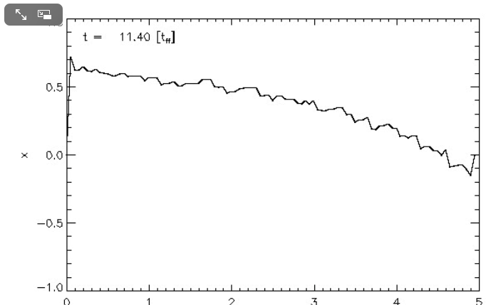 |
In an earlier paragraph, above, I pointed to Patrick's "time-dependent eigenfunction" animation (one frame, again, reprinted here on the right) and commented on how it should relate to the blue segment of the eigenfunction plots that I derived from linear perturbation theory (see Figure 6, above). The data that I have used to generate the blue segments for the models with <math>~\tilde\xi = 3.25</math> and <math>~\tilde\xi = 3.50</math> is provided in the pair of scrollable tables that I have added to the figure shown immediately above. For either model, the referenced blue segment can be generated by plotting x(renorm) vs. xi — i.e., using the first and third columns of either scrollable table — or by plotting x vs. xi — using the first and second columns of data. The only difference is that, in the x(xi) plot, x is normalized to unity at the surface of the model; in the x(renorm) vs. xi plot, x is normalized to unity at the center of the model.
Recommendation:
- Patrick could simply re-create the same linear-linear "time-dependent eigenfunction" movie, and add to every movie frame Joel's (time independent) blue segment eigenfunction; I guess, in this case, Joel's function should be normalized to unity at the center. Make sure that the normalization of the radius (horizontal axis) is the same in Patrick's time-dependent plots as it is in Joel's time-independent dataset.
- Patrick could generate a new eigenfunction movie in which the vertical axis is log-amplitude; Joel's time-independent eigenfunction should be added to every movie frame but, of course, in this case it should also be plotted as log-amplitude versus radius.
- Better yet, turn Joel's eigenfunction into a time-dependent eigenfunction! Using the evolutionary time that corresponds to each frame of the movie, multiply every x(xi) value by <math>~d_c \cdot e^{\sqrt{\omega^2}t}</math> with, I suppose, d_c = 1.5e-3. Using a semi-log diagram, plot this time-evolving curve on top of Patrick's numerically generated x(x_0,t) values and let's see how well they match over time!

|
|---|
|
© 2014 - 2021 by Joel E. Tohline |
