User:Tohline/2DStructure/ToroidalCoordinateIntegrationLimits

Toroidal-Coordinate Integration Limits

In support of our accompanying discussion of the gravitational potential of a uniform-density circular torus, here we explain in detail what limits of integration must be specified in order to accurately determine the volume — and, hence also the total mass — of such a torus using toroidal coordinates.

Mapping from Cylindrical to Toroidal Coordinates

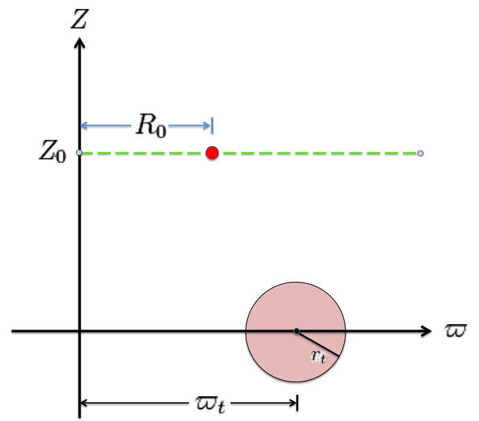
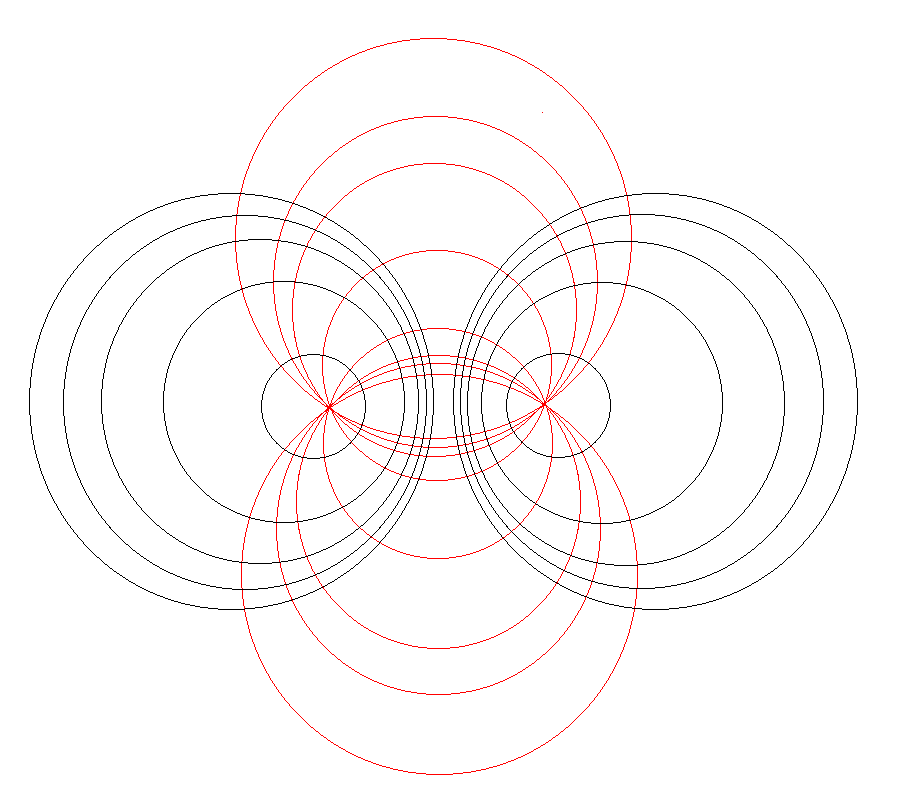
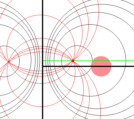
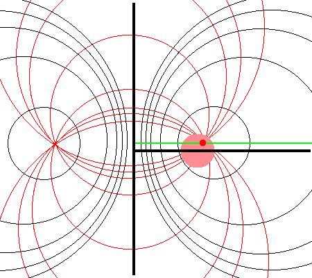
Referencing the illustration displayed in the left-hand panel of Figure 1, our goal is to determine the gravitational potential at any cylindrical-coordinate location <math>~(R_0, Z_0)</math> due to a uniform-density circular torus whose major radius is <math>~\varpi_t</math> and whose minor, cross-sectional radius is <math>~r_t</math>. Here we explain how a toroidal coordinate system <math>~(\xi_1, \xi_2)</math> — as defined, for example, by MF53 and as illustrated schematically in the right-hand panel of Figure 1 — can be used to reduce the geometric complexity of this problem. Note that, in our illustration, each black circle identifies a <math>\xi_1 = </math> constant surface and each red circle identifies a <math>\xi_2 = </math> constant surface. Note, as well, that the overall length scale (not labeled in our schematic diagram) is set by the distance, <math>~a</math>, from the vertical symmetry axis to the origin of the toroidal coordinate system — the point (actually, the axisymmetric ring) at which all the red circles intersect one another. Here we will show how, when using an appropriately aligned toroidal coordinate system, the three-dimensional, weighted integral over the mass distribution that is required to determine the gravitational potential at any location can be reduced to the sum of a small number (1 - 4) of one-dimensional integrals over the "radial" coordinate, <math>~\xi_1</math>.

Figure 1:    Meridional slice through …
(Pink) Circular Torus	Toroidal Coordinate System (schematic) (see also Wikipedia's Apollonian Circles)
The pink circle represents the meridional cross-section through an axisymmetric, circular torus that lies in the equatorial plane of a cylindrical <math>~(\varpi, Z)</math>, coordinate system. The torus has a major axis of length, <math>~\varpi_t</math>, and a minor, cross-sectional radius of length, <math>~r_t</math>. The red circular dot identifies the cylindrical-coordinate location, <math>~(R_0, Z_0)</math>, at which the gravitational potential is to be evaluated.	As is explained more fully in Wikipedia's discussion of toroidal coordinates, rotating this two-dimensional bipolar coordinate system about the vertical axis produces a three-dimensional toroidal coordinate system. Black circles centered on the horizontal axis become circular tori — each identifying an axisymmetric, <math>\xi_1 =</math> constant surface; whereas, red circles centered on the vertical axis become spheres — each identifying an axisymmetric, <math>\xi_2 =</math> constant surface.

Special Case Alignment

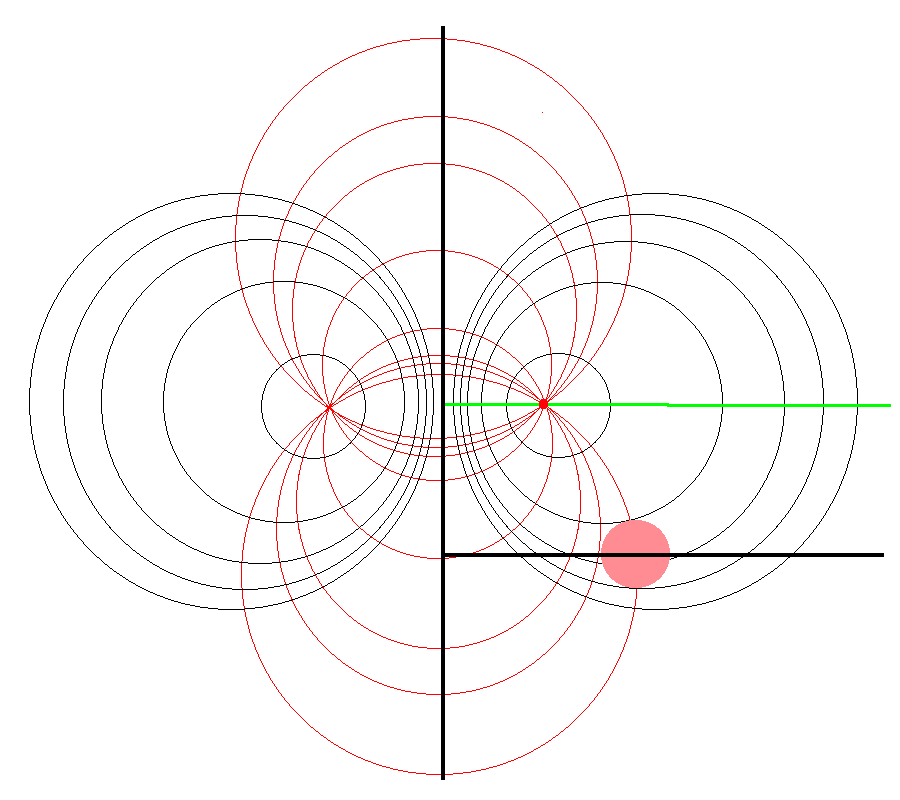
It should perhaps not be surprising to find that a toroidal coordinate system can be effectively used to quantitatively describe some properties — certainly the volume and possibly the gravitational potential — of circular tori because each <math>\xi_1 = </math> constant surface in a toroidal coordinate system (see the black circles in the right-hand panel of Figure 1) defines the surface of an axisymmetric, circular torus. In order to map from a cylindrical-coordinate representation of a circular torus (see the left-hand panel of Figure 1) to a toroidal-coordinate representation of that torus, at first glance it would seem reasonable to establish the alignment depicted schematically in Figure 2. That is, align the horizontal and vertical axes of the bipolar coordinate system (right-hand panel of Figure 1) with, respectively, the <math>\varpi-</math>axis and the <math>Z-</math>axis of the cylindrical coordinate system, then scale the overall size of the bipolar coordinate system until one <math>\xi_1 = </math> constant surface perfectly aligns with the surface of the (pink) torus.

Figure 2: Schematic Illustration of "Special Case" Alignment
Here, a mapping from cylindrical coordinates to toroidal coordinates is achieved by aligning the horizontal and vertical axes of the bipolar coordinate system (right-hand panel of Figure 1) with, respectively, the <math>\varpi-</math>axis and the <math>Z-</math>axis of the cylindrical coordinate system, then scaling the overall size of the bipolar coordinate system, <math>~a</math>, until one <math>\xi_1 = </math> constant surface perfectly aligns with the surface of the (pink) torus.

This is the "special case" alignment that we have discussed in an accompanying chapter. It is achieved by setting the scale-length, <math>~a</math>, of the toroidal-coordinate system to a value given by the expression,

<math>~a</math>

<math>~=</math>

<math>~\sqrt{\varpi_t^2 - r_t^2}\, ,</math>

which means that the "radial" toroidal coordinate that aligns with the surface of the (pink) torus has the value,

<math>~\xi_1</math>

<math>~=</math>

<math>~\frac{\varpi_t}{r_t} \, .</math>

While the special alignment depicted in Figure 2 might at first glance seem reasonable, we have found that it does not generally enable us to transform the multi-dimensional integral expression for the gravitational potential into a one-dimensional integral over <math>~\xi_1</math>, as desired.

Practical Transformation

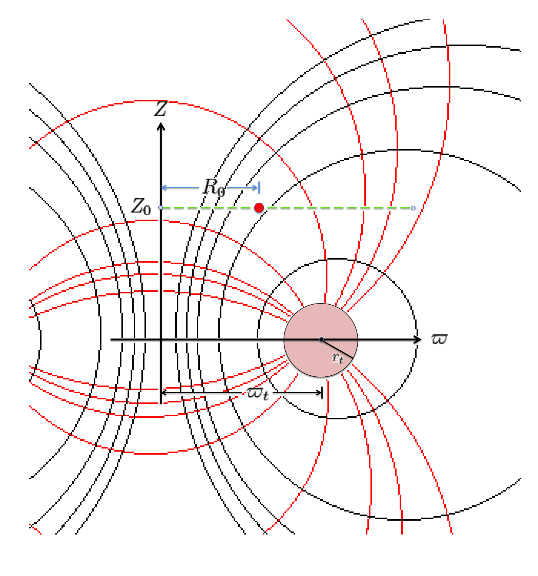
However, we have discovered that this desired transformation can be accomplished by shifting the toroidal-coordinate system vertically and scaling it such that its off-axis "origin" aligns with the cylindrical-coordinate location, <math>~(R_0, Z_0)</math>, at which the gravitational potential is to be evaluated. The left-hand panel of Figure 3 illustrates what results from aligning in this manner the left-hand and right-hand panels of Figure 1. The origin of the toroidal coordinate system sits on the green line-segment, a distance <math>~Z = Z_0</math> above the equatorial plane of the torus, and a distance <math>~a = R_0</math> from the symmetry axis.

Figure 3: Quantitative Illustration of Employed Toroidal Coordinate System

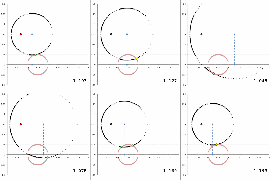
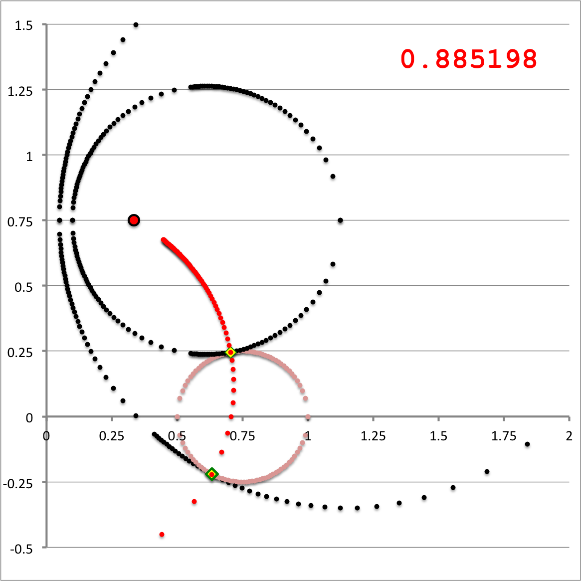
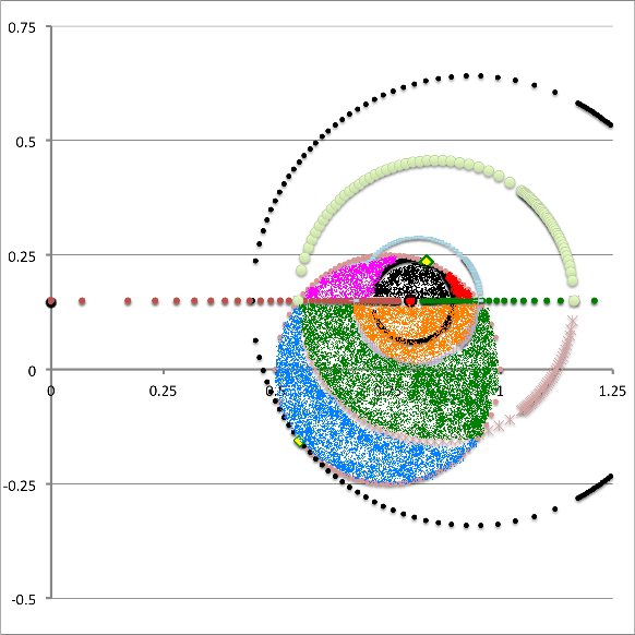
The middle and right-hand panels of Figure 3 display quantitatively how the boundary of the (pink) circular torus is defined in toroidal coordinates when an alignment of coordinate systems is made, as illustrated in the left-hand panel of Figure 3, for the parameter values: <math>~(R_0, Z_0) = (\tfrac{1}{3}, \tfrac{3}{4})</math> and <math>~(\varpi_t, r_t) = (\tfrac{3}{4}, \tfrac{1}{4})</math>. As the middle panel shows, black toroidal-coordinate circles intersect and/or thread through the (pink) torus for values of the radial coordinate in the range, <math>1.045 \leq \xi_1 \leq 1.193</math>. And, as the right-hand panel shows, the red toroidal-coordinate circle that corresponds to the angular-coordinate value, <math>~\xi_2 = 0.885198</math>, not only threads through the (pink) torus but identifies the "angle" at which the two limiting <math>\xi_1 =</math> constant circles touch the surface of the torus. The derivations that have led to the construction of these two figure panels are presented in an accompanying discussion.

One-Dimensional Integral Equations

Volume of Circular Torus

<math>~\frac{V_i}{V_\mathrm{torus}}</math> <math>~=</math> <math>~\frac{a^3}{2\pi \varpi_t r_t^2} \int\limits_{\xi_1 = \lambda_i}^{\xi_1 = \Lambda_i} d\xi_1 \biggl\{ \frac{(1-\xi_2^2)^{1/2} [ 4\xi_1^2 - 3\xi_1 \xi_2 - 1]}{(\xi_1^2-1)^2 (\xi_1 - \xi_2)^2} + \biggl[ \frac{(2\xi_1^2 + 1)}{(\xi_1^2-1)^{5/2}}\biggr] \cos^{-1}\biggl[ \frac{(\xi_1\xi_2 - 1 )}{(\xi_1- \xi_2)} \biggr] \biggr\}_{\xi_2 = \gamma_i}^{\xi_2 = \Gamma_i} \, . </math>

Note that when either integration limit, <math>~\gamma_i</math> or <math>~\Gamma_i</math>, is plus one, the integrand inside the curly braces becomes,

<math>~\biggl\{~~\biggr\}_{\xi_2 = +1}</math>

<math>~~\rightarrow~~</math>

<math>~ \biggl\{0 + \biggl[ \frac{(2\xi_1^2 + 1)}{(\xi_1^2-1)^{5/2}}\biggr] \cos^{-1}\biggl[ 1 \biggr] \biggr\} = 0 \, . </math>

Alternatively, when either integration limit, <math>~\gamma_i</math> or <math>~\Gamma_i</math>, is minus one, the integrand inside the curly braces becomes,

<math>~\biggl\{~~\biggr\}^{\xi_2 = -1}</math>

<math>~~\rightarrow~~</math>

<math>~ \biggl\{0 + \biggl[ \frac{(2\xi_1^2 + 1)}{(\xi_1^2-1)^{5/2}}\biggr] \cos^{-1}\biggl[- 1 \biggr] \biggr\} = \pi \biggl[ \frac{(2\xi_1^2 + 1)}{(\xi_1^2-1)^{5/2}}\biggr] \, . </math>

(In principle, the arccosine of -1 could be negative π, in which case the leading sign on this last expression should be flipped from positive to negative. But empirical evidence tells us that only the positive sign is relevant to this problem.)

Gravitational Potential due to a Circular Torus

<math>~\Phi_i(a,Z_0)</math> <math>~=</math> <math>~\frac{2^{5/2} G \rho_0 a^{2}}{3} \int\limits_{\xi_1 = \lambda_i}^{\xi_1 = \Lambda_i} \frac{(\xi_1+1)^{1/2}K(\mu) d\xi_1}{(\xi_1^2 - 1)^2 [ (\xi_1^2 - 1)^{1/2}+\xi_1 ]^{1/2} } \biggr[ \frac{\sin \theta(5\xi_1^2 - 4\xi_1 \cos \theta - 1)}{(\xi_1+1)^{1/2} (\xi_1 - \cos \theta)^{3/2}} </math>     <math>~ - 4\xi_1 E\biggl( \frac{\pi-\theta}{2} \, , \sqrt{\frac{2}{\xi_1 + 1}} \biggr) + (\xi_1-1) F\biggl( \frac{\pi-\theta}{2} \, , \sqrt{\frac{2}{\xi_1 + 1}} \biggr) \biggr]_{\theta = \cos^{-1}(\gamma_i)}^{\theta = \cos^{-1}(\Gamma_i)} \, . </math>

Evaluation of Elliptic Integrals

We use the Numerical Recipes algorithms to evaluate elliptic integrals; and we have checked our use of these algorithms against printed tables of elliptic integrals found in my CRC handbook. Here are the relevant steps used in confirming the proper evaluation of these functions.

First, my CRC handbook adopts the following notation (evaluating the incomplete elliptic integral of the first kind):

<math>~F(k,\phi) = \int_0^\phi \frac{d\Phi}{\sqrt{1 - k^2 \sin^2\Phi}}</math>

and

<math>~ \theta = \sin^{-1}k \, . </math>

Alternatively, in the Numerical Recipes algorithm, the two arguments of the incomplete elliptic integral of the first kind are, <math>~\mathrm{ellf}(\phi, k)</math>, where the relevant function expression is,

<math>~F(\phi,k)</math>

<math>~=</math>

<math>~ \int_0^\phi \frac{d\theta}{\sqrt{1 - k^2 \sin^2\theta}} \, , </math>

and the argument, <math>~\phi</math>, is expected to be provided in radians, instead of in degrees.

Some example values are:

Incomplete Elliptic Integrals of the First & Second Kind
CRC's    <math>~F(k,\phi)</math> (top);  <math>~E(k,\phi)</math> (bottom)							Numerical Recipe's    <math>~F(k,\phi)</math> (top); <math>~E(k,\phi)</math> (bottom)
<math>~\theta ~~ \rightarrow</math>	20°	35°	50°	65°	80°		<math>~k ~~ \rightarrow</math>	0.34202014	0.57357644	0.76604444	0.90630779	0.98480775
<math>~\phi</math>							<math>~\phi</math> (radians)
11°	0.1921	0.1924	0.1927	0.1930	0.1931		0.19198622	0.192123431 0.191849180	0.192373471 0.191600363	0.192679935 0.191296982	0.192961053 0.191020217	0.193140116 0.190844685
23°	0.4027	0.4049	0.4078	0.4105	0.4123		0.40142573	0.402656868 0.400201278	0.404940840 0.397964813	0.407815120 0.395213994	0.410528813 0.392680594	0.412298101 0.391061525
35°	0.6151	0.6231	0.6336	0.6441	0.6513		0.61086524	0.615064063 0.606716517	0.623082364 0.599066179	0.633639464 0.589516635	0.644149296 0.580570509	0.651323943 0.574768972
56°	0.9930	1.0250	1.0725	1.1285	1.1743		0.97738438	0.993020463 0.962159483	1.024993767 0.933452135	1.072482572 0.896220989	1.128479892 0.859487843	1.174295801 0.834363150
77°	1.3788	1.4554	1.5867	1.7909	2.0653		1.34390352	1.37884243 1.31035009	1.45540074 1.24566028	1.58672349 1.15795471	1.79094197 1.06431530	2.06528894 0.99170032
90° <math>~K(k)</math>	1.6200	1.7312	1.9356	2.3088	3.1534		π/2 <math>~K(k)</math>	1.	1.	1.	2.	3.

Integration Limits

We define the following terms that are functions only of the four principal model parameters, <math>~(a, Z_0, \varpi_t, r_t)</math>, and therefore can be treated as constants while carrying out the pair of nested integrals that determine <math>~q_0</math>.

Zone I:

Figure 4:  Zone I
Definition	Schematic Example
<math>~Z_0 > r_t</math> for any <math>~a</math>

In an accompanying discussion, we have derived the following integration limits; numerical values are given for the specific case, <math>~(a, Z_0, \varpi_t, r_t) = (\tfrac{1}{3}, \tfrac{3}{4}, \tfrac{3}{4}, \tfrac{1}{4})</math>:

<math>~\Lambda_1 = \xi_1|_\mathrm{max} </math> <math>~=</math> <math>~\biggl[1-\biggl( \frac{a}{\varpi_t-\beta_+} \biggr)^2 \biggr]^{-1/2} \approx 1.1927843</math> <math>~\lambda_1 = \xi_1|_\mathrm{min} </math> <math>~=</math> <math>~\biggl[1-\biggl( \frac{a}{\varpi_t-\beta_-} \biggr)^2 \biggr]^{-1/2} \approx 1.0449467</math>

where,

<math>~\kappa</math>	<math>~\equiv</math>	<math>~ Z_0^2 + a^2 - (\varpi_t^2 - r_t^2) </math>	<math>\rightarrow</math>	<math>~ \frac{5^2}{2^4\cdot 3^2} \approx 0.17361111 </math>
<math>~C</math>	<math>~\equiv</math>	<math>~1 + \biggl( \frac{2Z_0}{\kappa}\biggr)^2 ( \varpi_t^2 - r_t^2) </math>	<math>\rightarrow</math>	<math>~\frac{17 \cdot 1409}{5^4} \approx 38.3248 </math>
<math>~\beta_\pm</math>	<math>~\equiv</math>	<math>~ - \frac{\kappa}{2} \biggl[ \frac{\varpi_t \mp r_t \sqrt{C}}{(\varpi_t + r_t)(\varpi_t - r_t)} \biggr] </math>	<math>\rightarrow</math>	<math>~ -~\frac{5^2}{2^6\cdot 3}\biggl[ 1\mp \sqrt{ \frac{17\cdot 1409}{3^2\cdot 5^4}} \biggr] </math>

Notice that we have specified these integration limits such that, in going from the lower limit <math>~(\lambda_1)</math> to the upper limit <math>~(\Lambda_1)</math>, the value of <math>~\xi_1</math> monotonically increases. CAUTION: This statement is often not true. The quantity, <math>~\kappa</math>, changes signs, depending on whether <math>~(a^2 + Z_0^2) \gtrless (\varpi_t^2 -r_t^2)</math>. When <math>~\kappa</math> changes signs, the two quantities, <math>~\xi_1|_\mathrm{max}</math> and <math>~\xi_1|_\mathrm{min}</math> switch roles; specifically, <math>~\xi_1|_\mathrm{max}</math> becomes less than <math>~\xi_1|_\mathrm{min}</math> (or visa versa).

Also,

<math>~\Gamma_1 = \xi_2\biggr|_+</math> <math>~=</math> <math>~ \xi_1 - \frac{ (\xi_1^2-1)^{1/2}}{(\varpi_i/a)_+} </math> <math>~\gamma_1 = \xi_2\biggr|_-</math> <math>~=</math> <math>~ \xi_1 - \frac{ (\xi_1^2-1)^{1/2}}{(\varpi_i/a)_-} </math>

where, in addition to the quantities defined above,

<math>~\biggl(\frac{\varpi_i}{a}\biggr)_\pm</math>	<math>~\equiv</math>	<math>~\frac{\kappa}{2a^2}\cdot \frac{\mathrm{B}}{\mathrm{A}} \biggl[1 \pm \sqrt{1-\frac{AC}{B^2}} \biggr] </math>
<math>~\mathrm{A}</math>	<math>~\equiv</math>	<math>~\biggl(\frac{Z_0}{a}\biggr)^2 + \biggl[\frac{\varpi_t}{a} - \frac{\xi_1}{(\xi_1^2-1)^{1/2}}\biggr]^2 </math>
<math>~\mathrm{B}</math>	<math>~\equiv</math>	<math>~\biggl(\frac{2\varpi_t Z_0^2}{a\kappa}\biggr) - \biggl[\frac{\varpi_t}{a} - \frac{\xi_1}{(\xi_1^2-1)^{1/2}}\biggr] </math>

Here, our desire also is to specify the integration limits such that <math>~\xi_2</math> monotonically increases in going from the lower limit <math>~(\gamma_1)</math> to the upper limit <math>~(\Gamma_1)</math>. In order to check to see if this is the case, let's test the limiting values of <math>~\xi_2</math> when we are considering a radial-coordinate value roughly midway between its limits, say, when <math>~\xi_1 = 1.1</math>. For this specific case, we find,

<math>~\frac{\xi_1}{(\xi_1^2 - 1)^{1/2}} = 2.400397 \, ;</math>

<math>~\frac{\varpi_t}{a} - \frac{\xi_1}{(\xi_1^2-1)^{1/2}} = - 0.150397 \, ;</math>

<math>~A = 5.085119 \, ;</math>

<math>~B = 14.73040 \, ;</math>

<math>~\biggl(\frac{\varpi_i}{a}\biggr)_\pm = 2.263098\biggl[1 \pm \sqrt{1-0.898157} \biggr] \, ;</math>

<math>~\Rightarrow ~~~ \biggl(\frac{\varpi_i}{a}\biggr)_+ = 2.985318 \, ;</math>

<math>~\Rightarrow ~~~ \biggl(\frac{\varpi_i}{a}\biggr)_- = 1.540878 \, ;</math>

<math>~\Rightarrow ~~~ \xi_2\biggr|_+ = 0.946496 \, ;</math>

<math>~\Rightarrow ~~~ \xi_2\biggr|_- = 0.802600 \, .</math>

Hence, our ordering of the limits appears to be the one desired.

Zone II:

Figure 5:  Zone II
Definition	Schematic Example	Quantitative Example: Partial Volumes Identified
<math>~r_t > Z_0 > 0</math> and <math>~a < \varpi_t - \sqrt{r_t^2 - Z_0^2}</math>

In an accompanying discussion, we have derived the following integration limits; example numerical values of various parameters are provided for the specific case where, <math>~(a, Z_0, \varpi_t, r_t) = (\tfrac{1}{3}, \tfrac{3}{20}, \tfrac{3}{4}, \tfrac{1}{4})</math>. Note that,

<math>~\kappa</math>	<math>~=</math>	<math>~- \frac{1319}{2^4\cdot 3^2 \cdot 5^2} \approx -0.36639 \, ;</math>
<math>~C</math>	<math>~=</math>	<math>~1 + \frac{2^5\cdot 3^6 \cdot 5^2}{(1319)^2} = \frac{2322961}{(1319)^2} \approx 1.33522 \, ;</math>
<math>~\beta_+</math>	<math>~=</math>	<math>~\frac{1}{2^6\cdot 3^2\cdot 5^2} \biggl[3\cdot 1319 - \sqrt{2322961} \biggr] \approx 0.16895 \, ;</math>
<math>~\beta_-</math>	<math>~=</math>	<math>~\frac{1}{2^6\cdot 3^2\cdot 5^2} \biggl[3\cdot 1319 + \sqrt{2322961} \biggr] \approx 0.38063 \, .</math>

Partial Volume #II-1

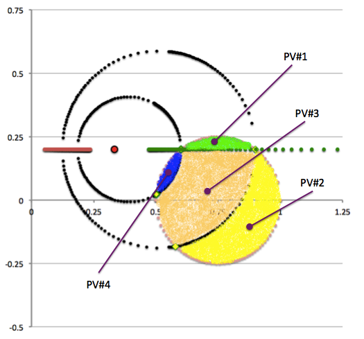
This is the green cropped-top sub-volume identified as Partial Volume #1 (PV#1) in the right-hand panel of Figure 5, and discussed in detail elsewhere.

<math>~\Lambda_1 </math> <math>~=</math> <math>~\frac{[\varpi_t - \sqrt{r_t^2 - Z_0^2}]^2 + a^2}{[\varpi_t - \sqrt{r_t^2 - Z_0^2}]^2-a^2} ~\rightarrow~\frac{1489}{13\cdot 53} \approx 2.16110</math> <math>~\lambda_1 </math> <math>~=</math> <math>~\frac{[\varpi_t + \sqrt{r_t^2 - Z_0^2}]^2 + a^2}{[\varpi_t + \sqrt{r_t^2 - Z_0^2}]^2-a^2} ~\rightarrow~ \frac{41\cdot 89}{7\cdot 11\cdot 37} \approx 1.28080</math>

<math>~\Gamma_1 = \xi_2\biggr|_+</math> <math>~=</math> <math>~ \xi_1 - \frac{ (\xi_1^2-1)^{1/2}}{(\varpi_i/a)_+} </math> <math>~\gamma_1 </math> <math>~=</math> <math>~1</math>

Partial Volume #II-2

This is the sub-volume that is painted yellow and identified as Partial Volume #2 (PV#2) in the right-hand panel of Figure 5.

<math>~\Lambda_2 </math> <math>~=</math> <math>~\frac{[\varpi_t + \sqrt{r_t^2 - Z_0^2}]^2 + a^2}{[\varpi_t + \sqrt{r_t^2 - Z_0^2}]^2-a^2} ~\rightarrow~ \frac{41\cdot 89}{7\cdot 11\cdot 37} \approx 1.28080</math> <math>~\lambda_2 </math> <math>~=</math> <math>~\xi_1|_\mathrm{max} = \biggl[1-\biggl( \frac{a}{\varpi_t-\beta_+} \biggr)^2 \biggr]^{-1/2} \approx 1.22088</math>

<math>~\Gamma_2 = \xi_2\biggr|_+</math> <math>~=</math> <math>~ \xi_1 - \frac{ (\xi_1^2-1)^{1/2}}{(\varpi_i/a)_+} </math> <math>~\gamma_2 = \xi_2\biggr|_-</math> <math>~=</math> <math>~ \xi_1 - \frac{ (\xi_1^2-1)^{1/2}}{(\varpi_i/a)_-} </math>

Partial Volume #II-3

This is the sub-volume that is painted orange and identified as Partial Volume #3 (PV#3) in the right-hand panel of Figure 5.

<math>~\Lambda_3 </math> <math>~=</math> <math>~\frac{[\varpi_t - \sqrt{r_t^2 - Z_0^2}]^2 + a^2}{[\varpi_t - \sqrt{r_t^2 - Z_0^2}]^2-a^2} ~\rightarrow~\frac{1489}{13\cdot 53} \approx 2.16110</math> <math>~\lambda_3 </math> <math>~=</math> <math>~\frac{[\varpi_t + \sqrt{r_t^2 - Z_0^2}]^2 + a^2}{[\varpi_t + \sqrt{r_t^2 - Z_0^2}]^2-a^2} ~\rightarrow~ \frac{41\cdot 89}{7\cdot 11\cdot 37} \approx 1.28080</math>

<math>~\Gamma_3 </math> <math>~=</math> <math>~ 1 </math> <math>~\gamma_3 = \xi_2\biggr|_-</math> <math>~=</math> <math>~ \xi_1 - \frac{ (\xi_1^2-1)^{1/2}}{(\varpi_i/a)_-} </math>

Partial Volume #II-4

This is the sub-volume that is painted blue and identified as Partial Volume #4 (PV#4) in the right-hand panel of Figure 5.

<math>~\Lambda_4 </math> <math>~=</math> <math>~\xi_1|_\mathrm{min} = \biggl[1-\biggl( \frac{a}{\varpi_t-\beta_-} \biggr)^2 \biggr]^{-1/2} \approx 2.32125</math> <math>~\lambda_4 </math> <math>~=</math> <math>~\frac{[\varpi_t - \sqrt{r_t^2 - Z_0^2}]^2 + a^2}{[\varpi_t - \sqrt{r_t^2 - Z_0^2}]^2-a^2} ~\rightarrow~\frac{1489}{13\cdot 53} \approx 2.16110</math>

<math>~\Gamma_4 = \xi_2\biggr|_+</math> <math>~=</math> <math>~ \xi_1 - \frac{ (\xi_1^2-1)^{1/2}}{(\varpi_i/a)_+} </math> <math>~\gamma_4 = \xi_2\biggr|_-</math> <math>~=</math> <math>~ \xi_1 - \frac{ (\xi_1^2-1)^{1/2}}{(\varpi_i/a)_-} </math>

Summary (Zone II)

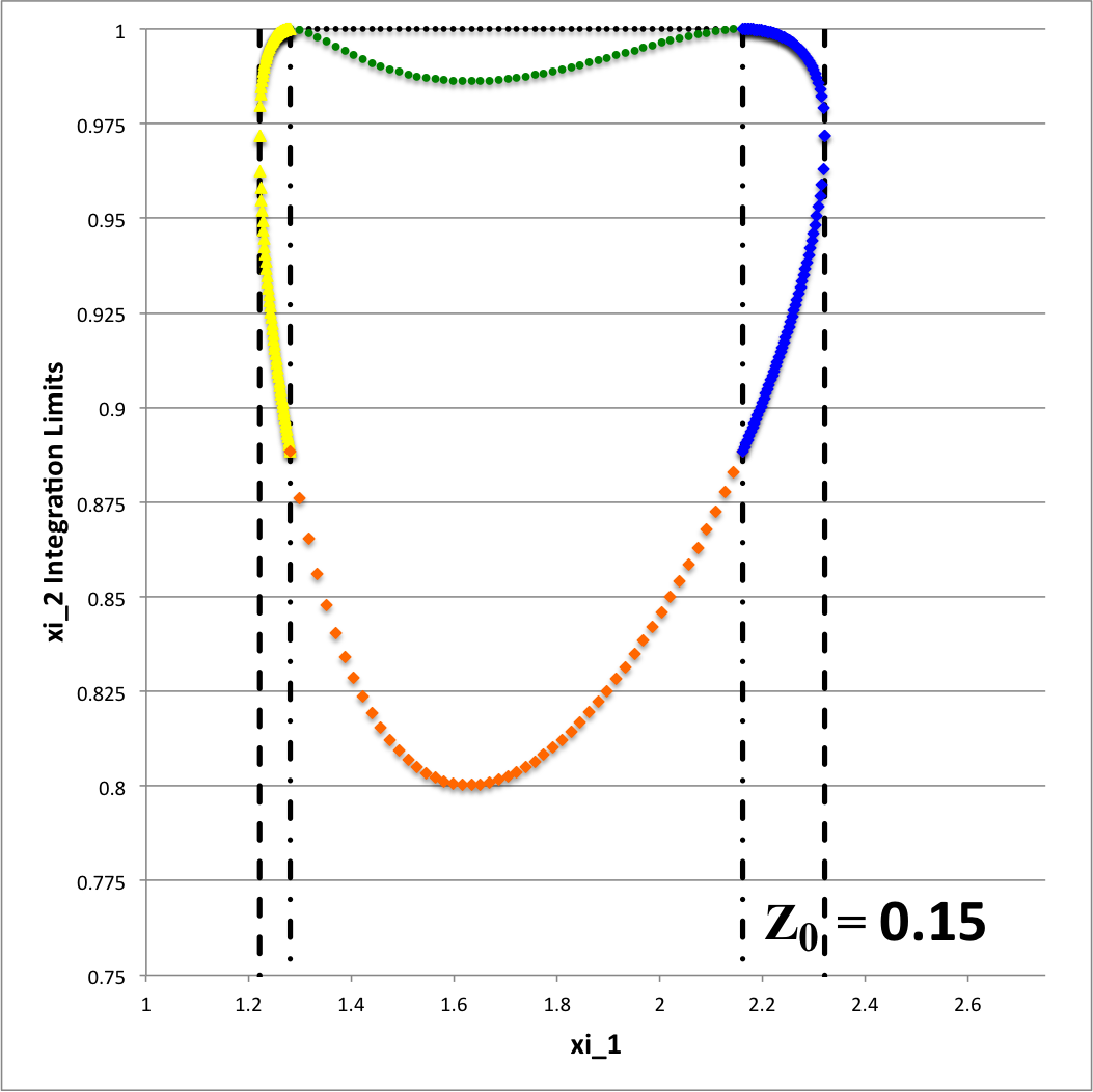
In summary, for a given set of the three model parameters <math>~(a, \varpi_t, r_t)</math> and the fourth, <math>~Z_0</math>, in the range, <math>~0 < Z_0 < r_t</math>, the volume of the (pink) circular torus is determined by adding together four partial volumes — that is, adding together the results of four separate 1D integrations over the "radial" toroidal coordinate <math>~(\xi_1)</math>. Although a total of eight radial integration limits (four lower limits and four upper limits) are required to fully determine the Zone II torus volume, only four unique limiting values need to be calculated because the partial volumes share <math>~\xi_1</math> boundaries. This has been illustrated by the black vertical dashed and dot-dashed lines in the left-hand panel of Figure 6 — and, drawing from the above discussion, the numerical values of these limits have been recorded in Table 1 — for the specific case of <math>~Z_0 = \tfrac{3}{20}</math>.

Table 1: Zone II Partial Volumes & Integration Limits on <math>~\xi_1</math> for model parameters <math>~(a, Z_0, \varpi_t, r_t) = (\tfrac{1}{3}, \tfrac{3}{20}, \tfrac{3}{4}, \tfrac{1}{4})</math>
	PV #1		PV #2		PV #3		PV #4
Integration Limits	<math>~\lambda_1</math>	<math>~\Lambda_1</math>	<math>~\lambda_2</math>	<math>~\Lambda_2</math>	<math>~\lambda_3</math>	<math>~\Lambda_3</math>	<math>~\lambda_4</math>	<math>~\Lambda_4</math>
	<math>2.16110</math>	<math>1.28080</math>	<math>1.28080</math>	<math>1.22088</math>	<math>2.16110</math>	<math>1.28080</math>	<math>2.32125</math>	<math>2.16110</math>
Volume Fraction	0.14237851		0.21569718		0.63537958		0.0065448719
Total Volume (nzones = 5000)	1.00000014       <math>~\Rightarrow~</math>      Error = -1.4E-7

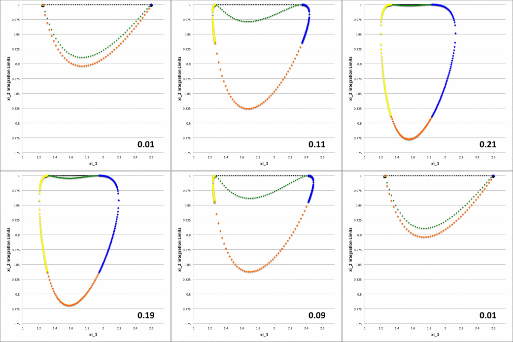
While the radial integrand expression for each partial volume is formally the same, it requires a specification of both limits, <math>~\gamma_i</math> and <math>~\Gamma_i</math>, for the "angular" coordinate integration which, as has also just been detailed, vary from one partial volume to the next and generally depend on the value of the radial coordinate. This dependence of the angular coordinate integration limits on the specific value of the radial coordinate across the four separate partial volumes is quantitatively illustrated in Figure 6 for the specific set of model parameters, <math>~(a, \varpi_t, r_t) = (\tfrac{1}{3}, \tfrac{3}{4}, \tfrac{1}{4})</math>, and for twenty-four different values of <math>~Z_0</math>.

Figure 6: Zone II Integration Limits on <math>~\xi_2</math> for model parameters <math>~(a, \varpi_t, r_t) = (\tfrac{1}{3}, \tfrac{3}{4}, \tfrac{1}{4})</math> and various <math>~Z_0</math>
Example <math>~\xi_2</math> Limits when <math>~Z_0 = \tfrac{3}{20} = 0.15</math> Partial Volume (i) Example <math>~\xi_1</math> <math>~\gamma_i</math> <math>~\Gamma_i</math> #1 2.00 1.00000 0.99625 #2 1.25 0.91635 0.99789 #3 2.00 0.84538 1.00000 #4 2.30 0.94684 0.98886

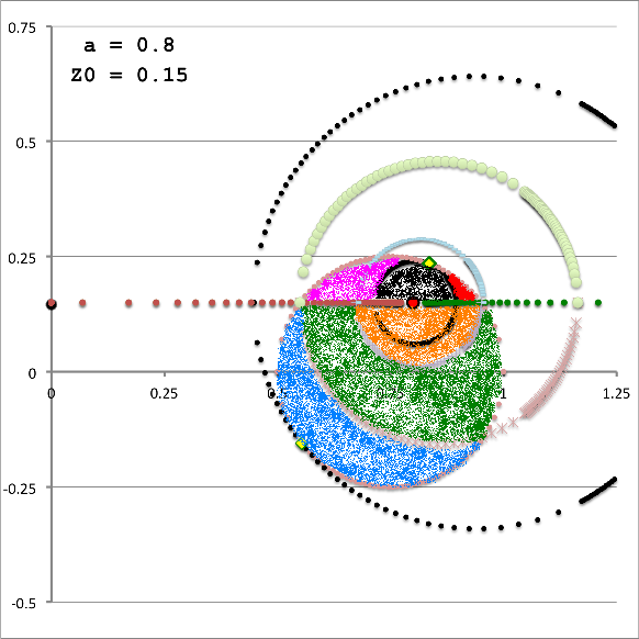
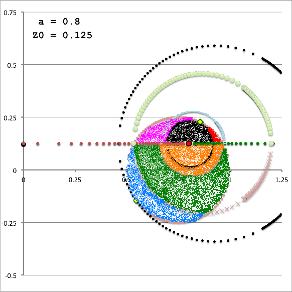
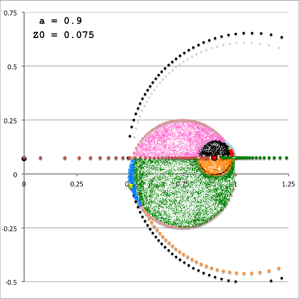
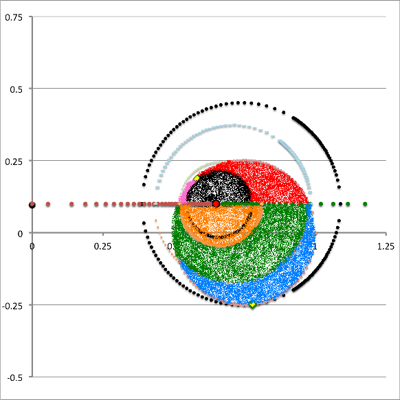
In both panels of Figure 6, at each of a variety of values of the "radial" coordinate, <math>~\xi_1</math> (horizontal axis), a pair of colored dots identify the values (vertical axis) of the two "angular" coordinate integration limits, <math>~\gamma_i</math> (lower value) and <math>~\Gamma_i</math> (upper value). The left-hand panel has been constructed for the specific case, <math>~Z_0 = \tfrac{3}{20} = 0.15</math>; via an animation sequence, the right-hand panel shows how the limits vary with <math>~\xi_1</math> for twenty-four different values of <math>~Z_0</math> in the Zone II range <math>~(0 \leq Z_0 \leq r_t)</math>, as indicated in the lower right-hand corner of each frame. The limits identified by yellow dots must be fed into the radial integrand expression when evaluating partial volume #2 and the blue dots provide the limits for partial volume #4. Green dots identify the lower angular-coordinate integration limit across partial volume #1; orange dots identify the lower limit across partial volume #3; and the upper limit for both partial volume #1 and partial volume #3 is unity (black dots). Four vertical black lines (two dashed and two dot-dashed) have been added to the plot displayed in the left-hand panel of Figure 6 in order to emphasize that the boundaries between the four partial volumes are defined by the radial-coordinate integration limits, <math>~\lambda_i</math> and <math>~\Lambda_i</math>; as has been detailed in Table 1 for the specific case <math>~(a, Z_0, \varpi_t, r_t) = (\tfrac{1}{3}, \tfrac{3}{20}, \tfrac{3}{4}, \tfrac{1}{4})</math>, the boundaries occur at <math>~\xi_1 = 1.22088, 1.28080, 2.16110,</math> and <math>~2.32125</math>.

Table 1b:  Validate Pattern II
Integration Limits for model parameters <math>~(a, Z_0, \varpi_t, r_t) = (\tfrac{4}{5}, \tfrac{3}{20}, \tfrac{3}{4}, \tfrac{1}{4})</math>
	<math>~\xi_1|_\mathrm{max}</math>	<math>~\xi_1|_\mathrm{min}</math>	<math>~\xi_1|_+</math>	<math>~\xi_1|_-</math>	<math>~\infty</math>
	1.22088	2.32125	1.28080	2.16110
<math>~\xi_2|_+</math>	END			START END
<math>~\xi_2|_-</math>		START	START	START
<math>~+1</math>			END END
<math>~-1</math>

Zone III

Figure 7:  Zone III
Definition	Schematic Example	Quantitative Example: Partial Volumes Identified
<math>~r_t > Z_0 > 0</math> and <math>~\varpi_t - \sqrt{r_t^2 - Z_0^2} < a < \varpi_t + \sqrt{r_t^2 - Z_0^2}</math> <math>~\biggl[\frac{11}{20} < a < \frac{19}{20}\biggr]</math>

Here, numerical values will be given for the specific case, <math>~(a, Z_0, \varpi_t, r_t) = (\tfrac{4}{5}, \tfrac{3}{20}, \tfrac{3}{4}, \tfrac{1}{4})</math>:

<math>~\xi_1|_\mathrm{max} </math> <math>~=</math> <math>~\biggl[1-\biggl( \frac{a}{\varpi_t-\beta_+} \biggr)^2 \biggr]^{-1/2} \approx 8.9243615</math> <math>~\xi_1|_\mathrm{min} </math> <math>~=</math> <math>~\biggl[1-\biggl( \frac{a}{\varpi_t-\beta_-} \biggr)^2 \biggr]^{-1/2} \approx 1.9116174</math>

where,

<math>~\kappa</math>	<math>~\equiv</math>	<math>~ Z_0^2 + a^2 - (\varpi_t^2 - r_t^2) </math>	<math>\rightarrow</math>	<math>~\frac{13}{2^4\cdot 5} = 0.1625 </math>
<math>~C</math>	<math>~\equiv</math>	<math>~1 + \biggl( \frac{2Z_0}{\kappa}\biggr)^2 ( \varpi_t^2 - r_t^2) </math>	<math>\rightarrow</math>	<math>\frac{457}{13^2} \approx 2.7041420 </math>
<math>~\beta_\pm</math>	<math>~\equiv</math>	<math>~ - \frac{\kappa}{2} \biggl[ \frac{\varpi_t \mp r_t \sqrt{C}}{(\varpi_t + r_t)(\varpi_t - r_t)} \biggr] </math>	<math>\rightarrow</math>	<math>~ -~\frac{1}{2^6\cdot 5 }\biggl[ 39 \mp \sqrt{457} \biggr] </math>
<math>~\Rightarrow~~~~\beta_+</math>	<math>\approx</math>	<math>~ -~0.055070130 </math>
<math>~\beta_-</math>	<math>\approx</math>	<math>~ -~0.188679870 </math>

Notice that we have specified these integration limits such that, in going from the lower limit <math>~(\lambda_1)</math> to the upper limit <math>~(\Lambda_1)</math>, the value of <math>~\xi_1</math> monotonically increases.

Partial Volume #III-1

This is the sub-volume that is painted blue and identified as Partial Volume #1 (PV#1) in the right-hand panel of Figure 7.

<math>~\Lambda_1 </math> <math>~=</math> <math>~\frac{a^2 + [\varpi_t - \sqrt{r_t^2 - Z_0^2}]^2}{a^2 - [\varpi_t - \sqrt{r_t^2 - Z_0^2}]^2} ~\rightarrow~ \frac{2^8+11^2}{2^8-11^2} \approx 2.79259</math> <math>~\lambda_1 </math> <math>~= </math> <math>~\xi_1|_\mathrm{min} = \biggl[1-\biggl( \frac{a}{\varpi_t-\beta_-} \biggr)^2 \biggr]^{-1/2} \approx 1.9116174</math>

<math>~\Gamma_1 = \xi_2\biggr|_+</math> <math>~=</math> <math>~ \xi_1 - \frac{ (\xi_1^2-1)^{1/2}}{(\varpi_i/a)_+} </math> <math>~\gamma_1 = \xi_2\biggr|_- </math> <math>~=</math> <math>~ \xi_1 - \frac{ (\xi_1^2-1)^{1/2}}{(\varpi_i/a)_-} </math>

Partial Volume #III-2

This is the sub-volume that is painted green and identified as Partial Volume #2 (PV#2) in the right-hand panel of Figure 7.

<math>~\Lambda_2 </math> <math>~=</math> <math>~\frac{[\varpi_t + \sqrt{r_t^2 - Z_0^2}]^2+a^2}{[\varpi_t + \sqrt{r_t^2 - Z_0^2}]^2-a^2} ~\rightarrow~ \frac{19^2 + 2^8}{19^2 - 2^8} \approx 5.87619</math> <math>~\lambda_2 </math> <math>~=</math> <math>~\frac{a^2 + [\varpi_t - \sqrt{r_t^2 - Z_0^2}]^2}{a^2 - [\varpi_t - \sqrt{r_t^2 - Z_0^2}]^2} ~\rightarrow~ \frac{2^8+11^2}{2^8-11^2} \approx 2.79259</math>

<math>~\Gamma_2 = \xi_2\biggr|_+</math> <math>~=</math> <math>~ \xi_1 - \frac{ (\xi_1^2-1)^{1/2}}{(\varpi_i/a)_+} </math> <math>~\gamma_2 </math> <math>~=</math> <math>~ -1 </math>

Partial Volume #III-3

This is the sub-volume that is painted orange and identified as Partial Volume #3 (PV#3) in the right-hand panel of Figure 7.

<math>~\Lambda_3 </math> <math>~=</math> <math>~\infty</math> <math>~\lambda_3 </math> <math>~=</math> <math>~\frac{[\varpi_t + \sqrt{r_t^2 - Z_0^2}]^2+a^2}{[\varpi_t + \sqrt{r_t^2 - Z_0^2}]^2-a^2} ~\rightarrow~ \frac{19^2 + 2^8}{19^2 - 2^8} \approx 5.87619</math>

<math>~\Gamma_3 </math> <math>~=</math> <math>~ +1 </math> <math>~\gamma_3 </math> <math>~=</math> <math>~ -1 </math>

Alternative determination of this partial volume:   Notice that this "orange" meridional-plane segment is a (semi)circle whose cross-sectional radius is (see accompanying discussion),

<math>~r_\mathrm{orange} = \frac{a}{\sqrt{\lambda_3^2 - 1}} \, ,</math>

and it is associated with a circular torus whose major radius is,

<math>~R_\mathrm{orange} = \lambda_3 r_\mathrm{orange} \, .</math>

Hence, using the familiar expression for the volume of a circular torus, we know that the volume associated with this "orange" partial volume is,

<math>~V_\mathrm{orange}</math>	<math>~=</math>	<math>~\frac{1}{2}\biggl[ 2\pi^2 R_\mathrm{orange} r_\mathrm{orange}^2 \biggr] = \pi^2 \lambda_3 r_\mathrm{orange}^3 = \frac{\pi^2 a^3 \lambda_3}{(\lambda_3^2-1)^{3/2}} </math>
<math>~\Rightarrow~~~~\frac{V_\mathrm{orange}}{V_\mathrm{torus}}</math>	<math>~=</math>	<math>~\biggl(\frac{a^3}{2\varpi_t r_t^2}\biggr) \frac{\lambda_3}{(\lambda_3^2-1)^{3/2}} \approx 0.165291952 \, .</math>

Partial Volume #III-4

This is the sub-volume that is painted pink and identified as Partial Volume #4a (PV#4a) in the right-hand panel of Figure 7.

<math>~\Lambda_4 </math> <math>~= </math> <math>~\xi_1|_\mathrm{max} = \biggl[1-\biggl( \frac{a}{\varpi_t-\beta_+} \biggr)^2 \biggr]^{-1/2} \approx 8.9243615</math> <math>~\lambda_4 </math> <math>~=</math> <math>~\frac{a^2 + [\varpi_t - \sqrt{r_t^2 - Z_0^2}]^2}{a^2 - [\varpi_t - \sqrt{r_t^2 - Z_0^2}]^2} ~\rightarrow~ \frac{2^8+11^2}{2^8-11^2} \approx 2.79259</math>

<math>~\Gamma_{4a} = \xi_2\biggr|_-</math> <math>~=</math> <math>~ \xi_1 - \frac{ (\xi_1^2-1)^{1/2}}{(\varpi_i/a)_-} </math> <math>~\gamma_{4a} </math> <math>~=</math> <math>~ -1 </math>

This is the sub-volume that is painted red and identified as Partial Volume #4b (PV#4b) in the right-hand panel of Figure 7.

<math>~\Lambda_4 </math> <math>~= </math> <math>~\xi_1|_\mathrm{max} = \biggl[1-\biggl( \frac{a}{\varpi_t-\beta_+} \biggr)^2 \biggr]^{-1/2} \approx 8.9243615</math> <math>~\lambda_4 </math> <math>~=</math> <math>~\frac{[\varpi_t + \sqrt{r_t^2 - Z_0^2}]^2+a^2}{[\varpi_t + \sqrt{r_t^2 - Z_0^2}]^2-a^2} ~\rightarrow~ \frac{19^2 + 2^8}{19^2 - 2^8} \approx 5.87619</math>

<math>~\Gamma_{4b} </math> <math>~=</math> <math>~ +1 </math> <math>~\gamma_{4b} = \xi_2\biggr|_+</math> <math>~=</math> <math>~ \xi_1 - \frac{ (\xi_1^2-1)^{1/2}}{(\varpi_i/a)_+} </math>

Partial Volume #III-5

This is the sub-volume that is painted black and identified as Partial Volume #5 (PV#5) in the right-hand panel of Figure 7.

<math>~\Lambda_5 </math> <math>~= </math> <math>~\infty</math> <math>~\lambda_5 </math> <math>~= </math> <math>~\xi_1|_\mathrm{max} = \biggl[1-\biggl( \frac{a}{\varpi_t-\beta_+} \biggr)^2 \biggr]^{-1/2} \approx 8.9243615</math>

<math>~\Gamma_{5} </math> <math>~=</math> <math>~ +1 </math> <math>~\gamma_{5} </math> <math>~=</math> <math>~ -1 </math>

Alternative determination of this partial volume:   Notice that this "black" meridional-plane segment is a (semi)circle whose cross-sectional radius is (see accompanying discussion),

<math>~r_\mathrm{black} = \frac{a}{\sqrt{\lambda_5^2 - 1}} \, ,</math>

and it is associated with a circular torus whose major radius is,

<math>~R_\mathrm{black} = \lambda_5 r_\mathrm{black} \, .</math>

Hence, using the familiar expression for the volume of a circular torus, we know that the volume associated with this "black" partial volume is,

<math>~V_\mathrm{black}</math>	<math>~=</math>	<math>~\frac{1}{2}\biggl[ 2\pi^2 R_\mathrm{black} r_\mathrm{black}^2 \biggr] = \pi^2 \lambda_5 r_\mathrm{black}^3 = \frac{\pi^2 a^3 \lambda_5}{(\lambda_3^2-1)^{3/2}} </math>
<math>~\Rightarrow~~~~\frac{V_\mathrm{black}}{V_\mathrm{torus}}</math>	<math>~=</math>	<math>~\biggl(\frac{a^3}{2\varpi_t r_t^2}\biggr) \frac{\lambda_5}{(\lambda_5^2-1)^{3/2}} \approx 0.06988365 \, .</math>

Summary (Zone III)

Table 2a:  Validate Pattern III-A
Integration Limits for model parameters <math>~(a, Z_0, \varpi_t, r_t) = (\tfrac{4}{5}, \tfrac{3}{20}, \tfrac{3}{4}, \tfrac{1}{4})</math>
	<math>~\xi_1|_\mathrm{max}</math>	<math>~\xi_1|_\mathrm{min}</math>	<math>~\xi_1|_+</math>	<math>~\xi_1|_-</math>	<math>~\infty</math>
	8.92436	1.91162	5.87619	2.79259
<math>~\xi_2|_+</math>	START	END		END
<math>~\xi_2|_-</math>				START END
<math>~+1</math>			END
<math>~-1</math>	START		START

Table 2b:  Validate Pattern III-A
Integration Limits for model parameters <math>~(a, Z_0, \varpi_t, r_t) = (\tfrac{4}{5}, \tfrac{1}{8}, \tfrac{3}{4}, \tfrac{1}{4})</math>
	<math>~\xi_1|_\mathrm{max}</math>	<math>~\xi_1|_\mathrm{min}</math>	<math>~\xi_1|_+</math>	<math>~\xi_1|_-</math>	<math>~\infty</math>
	7.19569	1.98820	5.35175	2.60173
<math>~\xi_2|_+</math>	START	END		END
<math>~\xi_2|_-</math>				START END
<math>~+1</math>			END
<math>~-1</math>	START		START

Table 2c:  Validate Pattern III-A
Integration Limits for model parameters <math>~(a, Z_0, \varpi_t, r_t) = (\tfrac{9}{10}, \tfrac{3}{40}, \tfrac{3}{4}, \tfrac{1}{4})</math>
	<math>~\xi_1|_\mathrm{max}</math>	<math>~\xi_1|_\mathrm{min}</math>	<math>~\xi_1|_+</math>	<math>~\xi_1|_-</math>	<math>~\infty</math>
	11.4106	1.84912	10.6947	1.95431
<math>~\xi_2|_+</math>	START	END		END
<math>~\xi_2|_-</math>				START END
<math>~+1</math>			END
<math>~-1</math>	START		START

Table 3a:  Validate Pattern III-B
Integration Limits for model parameters <math>~(a, Z_0, \varpi_t, r_t) = (\tfrac{13}{20}, \tfrac{1}{10}, \tfrac{3}{4}, \tfrac{1}{4})</math>
	<math>~\xi_1|_\mathrm{max}</math>	<math>~\xi_1|_\mathrm{min}</math>	<math>~\xi_1|_+</math>	<math>~\xi_1|_-</math>	<math>~\infty</math>
	2.10621	5.71122	2.57592	4.58888
Temporary	END	START START	END END START	END START
<math>~\xi_2|_+</math>	END	START
<math>~\xi_2|_-</math>			START	END START
<math>~+1</math>			END END
<math>~-1</math>		START

Table 4: Various Zone III Partial Volumes for model parameters <math>~(\varpi_t, r_t) = (\tfrac{3}{4}, \tfrac{1}{4})</math>
<math>~a</math>	<math>~Z_0</math>	nzones	PV#1 (blue)	PV#2 (green)	PV#3 (orange)	PV#4a (pink)	PV#4b (red)	PV#5 (black)	Error	Thumbnail
0.8	0.15	5000	(see Table 2 for details)						-1.1E-7
	0.10	5000	0.075401233	0.44164551	0.230637507	0.088778341	0.010790998	0.152746462	-4.8E-8
	0.125	5000	0.14811529	0.45526220	0.201121481	0.073678658	0.013215276	0.108607177	-8.7E-8
0.65	0.1	5000	0.21505365	0.38298966	0.149641005	0.0028992093	0.15531546	0.0941011094	-9.6E-8
0.9	0.075	5000	0.013247868	0.60594555	0.0688878257	0.25103223	0.00046944204	0.0604172907	-2.0E-7

September 2017

Coming Up to Speed

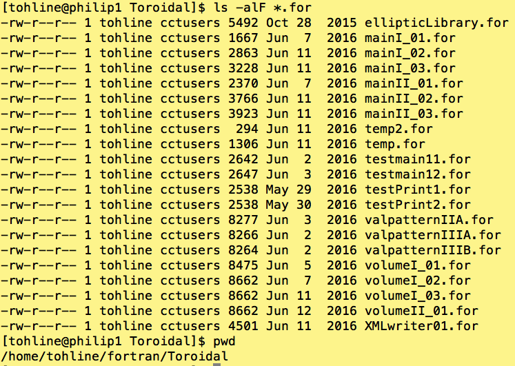
I am returning to this problem after letting it lay dormant for more than 14 months. These notes are being recorded as I try to decipher the fortran code that I have previously developed. Here is a screenshot from philip.hpc.lsu.edu that will help me archive the dates various fortran routines were last edited.

Let's start by reviewing the pair of routines (mainI_03.for,volumeI_03.for) which, presumably, integrate over the region labeled, Zone I, above.

Main Routine

Unedited mainI_03.for

Current Comments & Notes

June 12, 2016 ZoneI -- mainI_03.for (Generates good Vistrails error map.) ======================================== PROGRAM MainI real*8 dxx,dzz,dvarpi_t,dr_t,TorusPot,Volume,total,error real*8 p3,p5 real*8 griddx,Xstart,Xend,Ystart,Yend,gridedge real*8 x(49),y(49),xfull(50),yfull(50) real*8 e(49,49),esum real*8 elog real emax,emin real esumshort,elimit real eshort(49,49),xshort(50),yshort(50) integer iiZone,ngrid,i,j,k,ncount 151 format(1x,'Zone I:',5x,'Xstart, Xend, Ystart, Yend = ',& &1P4d14.5) 152 format(1x,' j ',' k ',7X,'x',14X,'y',10X,'error') 153 format(2I5,1p3d15.6) 154 format(5x,'Across ',I6,' zones, the average error = ',1p1d15.2) 601 format(1x,'emax, emin = ',1p2E15.3) dvarpi_t = 0.75d0 dr_t = 0.25d0 ngrid = 50 gridedge = 1.5d0 griddx = gridedge/dfloat(ngrid-1) xfull(1)=0.0d0 yfull(1)=0.0d0 do i=2,ngrid xfull(i) = xfull(i-1)+griddx yfull(i) = yfull(i-1)+0.5d0*griddx enddo x(1)=0.5d0*griddx y(1)=0.5d0*griddx do i=2,ngrid-1 x(i) = x(i-1)+griddx y(i) = y(i-1)+0.5d0*griddx enddo do j=1,ngrid-1 do k=1,ngrid-1 e(j,k)=0.0d0 enddo enddo !****** ! ! Zone I ! !****** ! [iiZone = 0] Full Volume ! iizone = 0 Xstart = 0.0d0 Xend = gridedge Ystart = dr_t Yend = y(ngrid-1)+0.5d0*griddx write(*,151)Xstart,Xend,Ystart,Yend write(*,152) ncount=0 esum=0.0d0 do k=1,ngrid-1 do j=1,ngrid-1 if(x(j).gt.Xstart .and. x(j).lt.Xend)then if(y(k).gt.Ystart .and. y(k).lt.Yend)then dxx = x(j) dzz = y(k) total = 0.0d0 call Integrate(dxx,dzz,dvarpi_t,dr_t,iiZone,TorusPot,Volume,p3,p5) e(j,k) = (1.0d0-Volume) ncount=ncount+1 esum = esum + DABS(e(j,k)) write(*,153)j,k,x(j),y(k),e(j,k) endif endif enddo enddo esum = esum/ncount write(*,154)ncount,esum ! Prepare for XMLwriter do k=1,ngrid xshort(k) = xfull(k) yshort(k) = yfull(k) enddo do k=1,ngrid-1 do j=1,ngrid-1 if(e(j,k).eq.0.0d0)e(j,k)=esum enddo enddo do k=1,ngrid-1 do j=1,ngrid-1 elog = dlog10(DABS(e(j,k))) eshort(j,k) = DABS(elog) enddo enddo emax = 0.0 emin = 20.0 esumshort = esum elimit = 1.5*esumshort do k=1,ngrid-1 do j=1,ngrid-1 if(eshort(j,k).gt.emax)emax=eshort(j,k) if(eshort(j,k).lt. emin)emin=eshort(j,k) if(eshort(j,k).lt.elimit)eshort(j,k)=elimit enddo enddo write(*,601)emax,emin do k=1,ngrid-1 do j=1,ngrid-1 eshort(j,k) = (eshort(j,k)-elimit)/(emax-elimit) enddo enddo emax = 0.0 emin = 20.0 do k=1,ngrid-1 do j=1,ngrid-1 if(eshort(j,k).gt.emax)emax=eshort(j,k) if(eshort(j,k).lt. emin)emin=eshort(j,k) enddo enddo write(*,601)emax,emin do k=1,ngrid-1 do j=1,ngrid-1 eshort(j,k) = (eshort(j,k)-emin)/(emax-emin) enddo enddo call XMLwriter01(ngrid,xshort,yshort,eshort) stop END PROGRAM MainI

dvarpi_t:   <math>~\varpi_t = \tfrac{3}{4}</math> dr_t:   <math>~r_t = \tfrac{1}{4}</math> (xfill, yfill) marks vertices, 1 --> ngrid = 50 (x, y) marks cell centers, 1 --> (ngrid-1) Rectilinear grid with <math>~\Delta x = \Delta y = 1.5/(50 - 1)</math> iiZone = 0 (Xstart, Xend, Ystart, Yend) = (0, 1.5, r_t, 1.5) (nested double) Loop through all cell centers that fall within these just-defined (X, Y) boundaries For each cell center: call Integrate calculate the "error", e = (1 - Volume) update the "counter", ncount = ncount + 1 add absolute value of the "error" to accumulated error, esum write: j, k, x, y, error esum = esum/ncount write: ncount, esum Arguments of Integrate(dxx,dzz,dvarpi_t,dr_t,iiZone,TorusPot,Volume,p3,p5) dxx:   cell-centered, x(j) dzz:   cell-centered, y(k) <math>~\varpi_t</math> <math>~r_t</math> iiZone Return:   TorusPot Return:   Volume p3 p5

Testing Volume Integration

Unedited volumeI_03.for	Current Comments & Notes
subroutine Integrate(RR,ZZ,v_t,r_t,iiZone,TorusPot,sumVol,pieceIII3,pieceIII5) !!!!!!!!!!!! ! ! Validate PATTERN III-B ! !!!!!!!!!!!! real*8 TorusPot,RR,ZZ,v_t,r_t real*8 kappa,C,betaPlus,betaMinus real*8 side,xi1Max,xi1Min real*8 xi1Plus,xi1Minus,xiStart,xiEnd real*8 grav,rho0,complete real completeS,muSingle real*8 Phi0,mu,coef,tempbeta,AAA,BBB real*8 viPlus,viMinus,xi2Plus,xi2Minus,thetaMax,thetaMin real*8 xx,ss,term1,darg1,darg2,tMax,tMin,sumPot real arg1,arg2 real*8 volMax,volMin,sumVol,Vol0,tempsum real*8 xi2One,xi2minOne,volOne,volminOne,volAdd real*8 xi(5000),xihalf(4999) real*8 pieceIII5,pieceIII3 integer n,idiag,nzones,iiZone 201 format(1x,'RR, ZZ, v_t, r_t:',1p4d13.5) 202 format(1x,'side, kappa, C, betaPlus, betaMinus, xi1Max, xi1Plus,& & xi1Minus, xi1Min') 203 format(1x, 1p9d13.5) idiag = 0 pii = 4.0d0*datan(1.0d0) complete = pii/2.0d0 completeS = complete grav = 1.0d0 rho0 = 1.0d0 Phi0 = 4.0d0*dsqrt(2.0d0)*grav*rho0*RR**2/3.0d0 Vol0 = 2.0d0*pii**2*v_t*r_t**2 side = (v_t**2 - r_t**2) kappa = ZZ**2 + RR**2 - side C = 1.0d0 + (2.0d0*ZZ/kappa)**2*side betaPlus = -(kappa/2.0d0)*(v_t - r_t*dsqrt(C))/side betaMinus = -(kappa/2.0d0)*(v_t + r_t*dsqrt(C))/side	grav --> <math>~G = 1</math> rho0 --> <math>~\rho_0 = 1</math> Phi0 = 4.0d0*dsqrt(2.0d0)*grav*rho0*RR**2/3.0d0 --> <math>~\frac{2^{5 / 2}}{3}\biggl(G\rho_0 R^2\biggr)</math> Vol0 = 2.0d0*pii**2*v_t*r_t**2     <math>~~~~\rightarrow ~~~~ 2\pi^2 \varpi_t r_t^2</math> side = (v_t**2 - r_t**2)     <math>~~~~\rightarrow~~~~ (\varpi_t^2 - r_t^2)</math> kappa = ZZ**2 + RR**2 - side     <math>~~~~\rightarrow~~~~ \kappa = Z^2 + R^2 - (\varpi_t^2 - r_t^2)</math> C = 1.0d0 + (2.0d0*ZZ/kappa)**2*side     <math>~\rightarrow~~~~ C = 1 + \biggl[\frac{2Z}{Z^2 + R^2 - (\varpi_t^2 - r_t^2)} \biggr]^2(\varpi_t^2 - r_t^2)</math> betaPlus = -(kappa/2.0d0)*(v_t - r_t*dsqrt(C))/side     <math>~\beta_+ = - \frac{\kappa (\varpi_t - r_t \sqrt{C})}{ 2(\varpi_t^2 - r_t^2)}</math> betaMinus = -(kappa/2.0d0)*(v_t + r_t*dsqrt(C))/side     <math>~\beta_- = - \frac{\kappa (\varpi_t + r_t \sqrt{C})}{ 2(\varpi_t^2 - r_t^2)}</math>
if(kappa.le.0.0d0)xi1Max = 1.0d0/dsqrt(1.0d0-(RR/(v_t-betaPlus))**2) if(kappa.gt.0.0d0)xi1Min = 1.0d0/dsqrt(1.0d0-(RR/(v_t-betaPlus))**2) pieceIII5 = RR**3*xi1Min/(2.0d0*v_t*r_t**2*(xi1Min**2-1.0d0)**1.5) if(kappa.le.0.0d0)xi1Min = 1.0d0/dsqrt(1.0d0-(RR/(v_t-betaMinus))**2) if(kappa.gt.0.0d0)xi1Max = 1.0d0/dsqrt(1.0d0-(RR/(v_t-betaMinus))**2) xi1Plus = 0.0d0 xi1Minus = 0.0d0 pieceIII3 = 0.0d0 if(r_t**2.ge.ZZ**2)then xi1Plus = DABS(((v_t + dsqrt(r_t**2 - ZZ**2))**2 + RR**2)/ & & ((v_t + dsqrt(r_t**2 - ZZ**2))**2 - RR**2)) endif if(r_t**2.ge.ZZ**2)then xi1Minus = DABS(((v_t - dsqrt(r_t**2 - ZZ**2))**2 + RR**2)/ & & ((v_t - dsqrt(r_t**2 - ZZ**2))**2 - RR**2)) endif if(r_t**2.ge.ZZ**2)then pieceIII3 = RR**3*xi1Minus/(2.0d0*v_t*r_t**2*(xi1Minus**2-1.0d0)**1.5) endif ! write(*,201)RR,ZZ,v_t,r_t ! write(*,202) ! write(*,203)side,kappa,C,betaPlus,betaMinus,xi1Max,xi1Plus,xi1Minus,xi1Min	<math>~\Rightarrow~~~\mathrm{pieceIII5} = \biggl(\frac{R^3 }{ 2\varpi_t r_t^2}\biggr) \biggl[ 1 - \frac{R^2}{(\varpi_t - \beta_-)^2} \biggr]^{-1 / 2} \biggl\{ \biggl[ 1 - \frac{R^2}{(\varpi_t - \beta_-)^2} \biggr]^{-1 / 2} - 1 \biggr\}^{- 3 / 2}</math>       <math>~\xi_1|_\mathrm{min}</math> <math>~\xi_1|_\mathrm{max}</math> <math>~\kappa \le 0</math> <math>~\biggl[ 1 - \frac{R^2}{(\varpi_t - \beta_-)^2} \biggr]^{-1 / 2}</math> <math>~\biggl[ 1 - \frac{R^2}{(\varpi_t - \beta_+)^2} \biggr]^{-1 / 2}</math> <math>~\kappa > 0</math> <math>~\biggl[ 1 - \frac{R^2}{(\varpi_t - \beta_+)^2} \biggr]^{-1 / 2}</math> <math>~\biggl[ 1 - \frac{R^2}{(\varpi_t - \beta_-)^2} \biggr]^{-1 / 2}</math>       <math>~\xi_1|_-</math> <math>~\xi_1|_+</math> pieceIII3 <math>~r_t^2 < Z^2</math> <math>~0</math> <math>~0</math> <math>~0</math> <math>~r_t^2 \ge Z^2</math> <math>~~~ \biggl| \frac{ \varpi_t - \sqrt{(r_t^2 - Z^2)^2 + R^2} }{ \varpi_t - \sqrt{ (r_t^2 - Z^2)^2 - R^2 } } \biggr|~~~</math> <math>~~~\biggl| \frac{ (\varpi_t + \sqrt{ r_t^2 - Z^2})^2 + R^2 }{ ( \varpi_t + \sqrt{r_t^2 - Z^2 } )^2 - R^2} \biggr|~~~</math> <math>~R^3 \xi_1|_- \biggl[ 2\varpi_t r_t^2 ( \xi^2_1|_- - 1)^{3 / 2}\biggr]^{- 1}</math>
! Begin 1D integration ! Specify sub-region... !!!!!!!!!!!!!!!!!!!!!!!!!!!!!!! ! ! On 29 May 2016, modified iiZone definition to correspond with ! online VisTrails chapter discussion: ! User:Tohline/2DStructure/ToroidalCoordinateIntegrationLimits ! !!!!!!!!!!!!!!!!!!!!!!!!!!!!!!! ! ! ZONE II ! [iiZone = 1] Green cropped-top sub-volume if(iiZone .eq. 1)then xi1Start = xi1Minus xi1End = xi1Plus ! [iiZone = 3] Lower (orange) Sub-volume that shares edge with ! Green cropped-top sub-volume else if(iiZone .eq. 3)then xi1Start = xi1Minus xi1End = xi1Plus ! [iiZone = 4] (Blue) Segment to the left of Lower Sub-volume else if(iiZone .eq. 4)then xi1Start = xi1Min xi1End = xi1Minus ! [iiZone = 2] (Yellow) Segment to the right of Lower Sub-volume else if(iiZone .eq. 2)then xi1Start = xi1Plus xi1End = xi1Max ! ! ZONE III ! [iiZone = 31] (lightblue) Segment of Zone III else if(iiZone .eq. 31)then xi1End = xi1Max xi1Start = xi1Plus ! [iiZone = 32] (darkgreen) Segment of Zone III else if(iiZone .eq. 32)then xi1End = xi1Plus xi1Start = xi1Minus ! [iiZone = 33] (pink=4a) Segment of Zone III else if(iiZone .eq. 33)then xi1End = xi1Plus xi1Start = xi1Min ! [iiZone = 34] (red=4b) Segment of Zone III else if(iiZone .eq. 34)then xi1End = xi1Minus xi1Start = xi1Min ! ! ZONE I ! Full volume else xi1Start = xi1Min xi1End = xi1Max end if ! Finished specifying sub-region	Next comments.
sumPot = 0.0d0 sumVol = 0.0d0 nzones = 1000 dxi = (xi1End-xi1Start)/dfloat(nzones-1) xi(1) = xi1Start do n=2,nzones xi(n) = xi(n-1)+dxi end do do n=1,nzones-1 xihalf(n) = 0.5d0*(xi(n) + xi(n+1)) end do ! For each value of xi, evaluate these quantities !!!!Diagnostics!!!! 303 format(1x,'arg1 = ',1pd15.7,/,& & 1x,'arg2 = ',1pd15.7,/,& & 1x,'tMax = ',1pd15.7,/) 304 format(1x,'arg1 = ',1pd15.7,/,& & 1x,'arg2 = ',1pd15.7,/,& & 1x,'tMin = ',1pd15.7,/) 403 format(1x,'arg1 = ',1pd15.7,/,& & 1x,'volMax = ',1pd15.7,/) 404 format(1x,'arg1 = ',1pd15.7,/,& & 1x,'volMin = ',1pd15.7,/) 405 format(1x,'TorusPot = ',1pd15.7,/,& & 1x,'sum = ',1pd15.7,/,& & 1x,'Vol0 = ',1pd15.7,/,& & 1x,'sumVol = ',1pd15.7,/) ! If Z0 less than radius of torus, carry out double integration do n=1,nzones-1 xx = xihalf(n) ! xx = xi(n) ss = dsqrt(xx**2-1.0d0) mu = dsqrt(2.0d0*ss/(ss+xx)) muSingle = mu ! coef = dsqrt(xx+1)*ellf(completeS,muSingle)/(ss**4*dsqrt(ss+xx)) coef = 1.0d0 tempbeta = v_t/RR - xx/ss AAA = (ZZ/RR)**2 + tempbeta**2 BBB = 2.0d0*v_t*ZZ**2/(RR*kappa) - tempbeta term1 = 1.0d0 - AAA*C/BBB**2 if(term1.lt.0.0d0)term1=0.0d0 viPlus = kappa*BBB/(2.0d0*RR**2*AAA)*(1.0d0+dsqrt(term1)) viMinus = kappa*BBB/(2.0d0*RR**2*AAA)*(1.0d0-dsqrt(term1)) xi2Plus = xx - ss/viPlus xi2Minus = xx - ss/viMinus thetaMax = dacos(xi2Plus) thetaMin = dacos(xi2Minus) darg2 = dsqrt(2.0d0/(1.0d0+xx)) arg2 = darg2 ! Determine T(thetaMax)... ! darg1 = (pii - thetaMax)/2.0d0 ! arg1 = darg1 ! tMax = dsin(thetaMax)*(5.0d0*xx**2 - 4.0d0*xx*xi2Plus - 1.0d0)& ! & /(dsqrt(xx + 1.0d0)*dsqrt((xx-xi2Plus)**3))& ! & -4.0d0*xx*elle(arg1,arg2) + (xx-1.0d0)*ellf(arg1,arg2) ! write(*,310)ss,mu,tempbeta,AAA,BBB,viPlus,viMinus 310 format(1x,'ss, mu, tempbeta, AAA, BBB, viPlus, viMinus:',& & /,1x,1p7d15.7) ! write(*,303)arg1,arg2,tMax ! Determine T(thetaMin)... ! darg1 = (pii - thetaMin)/2.0d0 ! arg1 = darg1 ! tMin = dsin(thetaMin)*(5.0d0*xx**2 - 4.0d0*xx*xi2Minus - 1.0d0)& ! & /(dsqrt(xx + 1.0d0)*dsqrt((xx-xi2Minus)**3))& ! & -4.0d0*xx*elle(arg1,arg2) + (xx-1.0d0)*ellf(arg1,arg2) ! write(*,304)arg1,arg2,tMin !! ! sumPot = sumPot + dxi*coef*(tMax - tMin) ! TORUS VOLUME DETERMINATION... xi2One = 1.0d0 xi2minOne = -1.0d0 ! Determine Vol(thetaMax)... volMax = dsqrt(1.0d0-xi2Plus**2)*(4.0d0*xx**2 - 3.0d0*xx*xi2Plus - 1.0d0)& & /(ss**4*(xx-xi2Plus)**2)& & + ((2.0d0*xx**2+1.0d0)/ss**5)*dacos((xx*xi2Plus - 1.0d0)/(xx-xi2Plus)) ! Determine Vol(thetaMin)... volMin = dsqrt(1.0d0-xi2Minus**2)*(4.0d0*xx**2 - 3.0d0*xx*xi2Minus - 1.0d0)& & /(ss**4*(xx-xi2Minus)**2)& & + ((2.0d0*xx**2+1.0d0)/ss**5)*dacos((xx*xi2Minus - 1.0d0)/(xx-xi2Minus)) ! Determine Vol(One)... volOne = 0.0 ! volOne = dsqrt(1.0d0-xi2One**2)*(4.0d0*xx**2 - 3.0d0*xx*xi2One - 1.0d0)& ! & /(ss**4*(xx-xi2One)**2)& ! & + ((2.0d0*xx**2+1.0d0)/ss**5)*dacos((xx*xi2One - 1.0d0)/(xx-xi2One)) ! Determine Vol(minusOne)... volminOne = pii*((2.0d0*xx**2+1.0d0)/ss**5) ! volminOne = dsqrt(1.0d0-xi2minOne**2)*(4.0d0*xx**2 - 3.0d0*xx*xi2minOne - 1.0d0)& ! & /(ss**4*(xx-xi2minOne)**2)& ! & + ((2.0d0*xx**2+1.0d0)/ss**5)*dacos((xx*xi2minOne - 1.0d0)/(xx-xi2minOne)) ! Specify sub-region... ! Full volume or similar segments ... if(iiZone.eq.0 .or. iiZone.eq.2 .or. iiZone.eq.4)volAdd = volMax-volMin ! [iiZone = 1] Green cropped-top sub-volume if(iiZone .eq. 1)volAdd = volOne - volMax ! [iiZone = 2] Lower (orange) Sub-volume that shares edge with Green cropped-top sub-volume if(iiZone .eq. 3)volAdd = volOne-VolMin ! [iiZone = 31] Blue sub-volume of zone III if(iiZone.eq.31)volAdd = volMax - volMin ! [iiZone = 32 ] Darkgreen Sub-volumes of zone III if(iiZone .eq. 32)volAdd = volOne - volMin ! [iiZone = 33] Pink Sub-volumes of zone III if(iiZone .eq. 33)volAdd = volOne - volMax ! [iiZone = 34] Red Sub-volume zone III if(iiZone .eq. 34)volAdd = volMin - volminOne sumVol = sumVol + dxi*volAdd enddo tempsum = sumVol sumVol = pii*RR**3*sumVol/Vol0 ! write(*,405)TorusPot,tempsum,Vol0,sumVol return end	Next comments.

XML Writer for Visualization

Unedited XMLwriter01.for

Current Comments & Notes

Subroutine XMLwriter01(imax,x,y,cell_scalar) real x(50),y(50),z(1) real cell_scalar(49,49),point_scalar(50,50) integer imax integer extentX,extentY,extentZ integer ix0,iy0,iz0 integer norm(50,3) ! imax=50 ix0=0 iy0=0 iz0=0 extentX=imax-1 extentY=imax-1 extentZ=0 z(1) = 0.0 ! Set normal vector 1D array do i=1,imax norm(i,1)=0 norm(i,2)=0 norm(i,3)=1 enddo ! Set values of point_scalar array do i=1,imax-1 do j=1,imax-1 point_scalar(i,j)=cell_scalar(i,j) enddo enddo do i=1,imax-1 point_scalar(i,imax)=cell_scalar(i,imax-1) enddo do j=1,imax-1 point_scalar(imax,j)=cell_scalar(imax-1,j) enddo point_scalar(imax,imax)=point_scalar(imax-1,imax) ! End point_scalar definition 201 format('<?xml version="1.0"?>') 202 format('<VTKFile type="RectilinearGrid" version="0.1" byte_order="LittleEndian">') 302 format('</VTKFile>') 203 format(2x,'<RectilinearGrid WholeExtent="',6I3,'">') 303 format(2x,'</RectilinearGrid>') 204 format(4x,'<Piece Extent="',6I3,'">') 304 format(4x,'</Piece>') 205 format(6x,'<CellData Scalars="cell_scalars" Normals="magnify">') 305 format(6x,'</CellData>') 206 format(8x,'<DataArray type="Float32" Name="magnify" NumberOfComponents="3" format="ascii">') 207 format(8x,'<DataArray type="Float32" Name="cell_scalars" format="ascii">') 399 format(8x,'</DataArray>') 208 format(6x,'<PointData Scalars="colorful" Normals="direction">') 308 format(6x,'</PointData>') 209 format(8x,'<DataArray type="Float32" Name="colorful" format="ascii">') 210 format(6x,'<Coordinates>') 310 format(6x,'</Coordinates>') 211 format(8x,'<DataArray type="Float32" format="ascii" RangeMin="0" RangeMax="5">') 212 format(8x,'<DataArray type="Float32" format="ascii">') 213 format(8x,'<DataArray type="Float32" Name="direction" NumberOfComponents="3" format="ascii">') 501 format(10f9.5) 502 format(10f9.5) 503 format(5x,9(1x,3I2)) 504 format(10f9.5) 505 format(5x,10(1x,3I2)) !!!!! ! ! Begin writing out XML tags. ! !!!!! write(*,201)  !<?xml write(*,202) !VTKFile write(*,203)ix0,extentX,iy0,extentY,iz0,extentZ  ! RectilinearGrid write(*,204)ix0,extentX,iy0,extentY,iz0,extentZ  ! Piece write(*,205)  ! CellData write(*,207)  ! DataArray(cell_scalars) do j=1,imax-1 write(*,501)(cell_scalar(i,j),i=1,imax-1) enddo write(*,399)  ! /DataArray write(*,206)  ! DataArray(cell_scalars) do j=1,imax-1 write(*,503)(norm(i,1),norm(i,2),norm(i,3),i=1,imax-1) enddo write(*,399)  ! /DataArray write(*,305)  ! /CellData write(*,208)  ! PointData write(*,209)  ! DataArray(points) write(*,502)((point_scalar(i,j),j=1,imax),i=1,imax) write(*,399)  ! /DataArray write(*,213)  ! DataArray(cell_scalars) do j=1,imax write(*,505)(norm(i,1),norm(i,2),norm(i,3),i=1,imax) enddo write(*,399)  ! /DataArray write(*,308)  ! /PointData write(*,210)  ! Coordinates write(*,212)  ! DataArray(x-direction) write(*,504)(x(i),i=1,imax) write(*,399)  ! /DataArray write(*,212)  ! DataArray(y-direction) write(*,504)(y(i),i=1,imax) write(*,399)  ! /DataArray write(*,212)  ! DataArray(z-direction) write(*,504)z(1) write(*,399)  ! /DataArray write(*,310)  ! /Coordinates write(*,304)  ! /Piece write(*,303)  ! /RectilinearGrid write(*,302)  !/VTKFile return end

dvarpi_t:   <math>~\varpi_t = \tfrac{3}{4}</math>

See Also

• Wikipedia's discussion of Toroidal Coordinates
• Determining the Gravitational Potential Using Toroidal Coordinates
• Ramblings Appendix Chapter: Determining the Relationships between Toroidal Coordinates and other Coordinate Systems

 

© 2014 - 2021 by Joel E. Tohline |   H_Book Home   |   YouTube   | Appendices: | Equations | Variables | References | Ramblings | Images | myphys.lsu | ADS | Recommended citation:   Tohline, Joel E. (2021), The Structure, Stability, & Dynamics of Self-Gravitating Fluids, a (MediaWiki-based) Vistrails.org publication, https://www.vistrails.org/index.php/User:Tohline/citation