Difference between revisions of "User:Tohline/SSC/Structure/BiPolytropes/MurphyUVplane"
(Begin constructing table to critique Murphy's analysis) |
(→Critique of Murphy's Model Characteristics: Insert long multi-colored table from separate chapter) |
||
| (6 intermediate revisions by the same user not shown) | |||
| Line 290: | Line 290: | ||
<font color="red">'''CAUTION:'''</font> Presented in this fashion — that is, by using <math>~\xi</math> to represent the dimensionless radial coordinate in all four expressions — Murphy's expressions seem to imply that the independent variable defining the radial coordinate in the bipolytrope's core is the same as the one that defines the radial coordinate in the structure's envelope. In general, this will not be the case, so we have explicitly used a different independent variable, <math>~\eta</math>, to mark the envelope's radial coordinate in our expressions. It is clear from other elements of his published derivation that Murphy understood this distinction but, as is explained more fully below, errors in his final model specifications may have resulted from not explicitly differentiating between this variable notation. | <font color="red">'''CAUTION:'''</font> Presented in this fashion — that is, by using <math>~\xi</math> to represent the dimensionless radial coordinate in all four expressions — Murphy's expressions seem to imply that the independent variable defining the radial coordinate in the bipolytrope's core is the same as the one that defines the radial coordinate in the structure's envelope. In general, this will not be the case, so we have explicitly used a different independent variable, <math>~\eta</math>, to mark the envelope's radial coordinate in our expressions. It is clear from other elements of his published derivation that Murphy understood this distinction but, as is explained more fully below, errors in his final model specifications may have resulted from not explicitly differentiating between this variable notation. | ||
==Critique of Murphy's Model Characteristics== | |||
{{LSU_WorkInProgress}} | |||
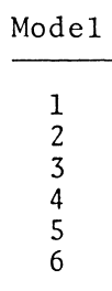
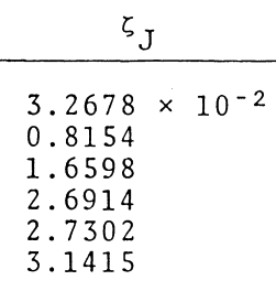
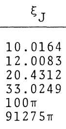
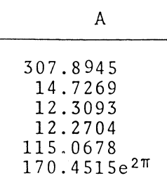
As a supplement to the preceding two figures, the following table shows in quantitative detail how we are able to ''analytically'' derive individual coordinate roots, <math>~(A_0\eta)_\mathrm{root}</math> — see the next-to-last column of the table — from ten different interface-coordinate locations, <math>~\xi_i = \zeta_J</math>, as specified in the first (left-most) column of the table. The interface parameter, <math>~\kappa_i</math>, is determined directly from the specified value of <math>~\xi_i</math>; the parameter, <math>~p=(1-\kappa_i)^{-1}</math>; then, given <math>~p</math>, the root to the cubic equation and, in turn, the value of <math>~\Delta_i</math>, are determined; and, finally, a choice of the integer phase-shift parameter, <math>~m</math>, leads to the calculation of <math>~(A_0\eta)_\mathrm{root}</math>. For comparison, the last (right-most) column of the table lists the corresponding coordinate, <math>~\xi_J</math>, as originally derived and published by [http://adsabs.harvard.edu/abs/1983PASAu...5..175M Murphy (1983)]. Coordinate pairs shown in the orange-colored panels of our table correspond to the six models whose characteristics are provided in Murphy's Table 3; coordinate pairs shown in the green-colored panels correspond to two of the ten "F2 = 0" roots identified in Murphy's Table 1; and the additional three coordinate pairs shown in the blue-colored panels have been drawn from Murphy's Table 2. | |||
<div align="center"> | |||
<table border="1" cellpadding="7"> | |||
<tr> | |||
<td align="center" rowspan="2"> | |||
Murphy (1983) | |||
Tables 1, 2, & 3 | |||
</td> | |||
<td align="center" colspan="6"> | |||
Here … setting <math>\xi_i = \zeta_J</math> … and assuming <math>\mu_e/\mu_c = 1</math> | |||
</td> | |||
<td align="center" rowspan="2"> | |||
Murphy (1983) | |||
Tables 1, 2, & 3 | |||
</td> | |||
</tr> | |||
<tr> | |||
<td align="center" colspan="6"> | |||
1<sup>st</sup> Constraint | |||
</td> | |||
</tr> | |||
<tr> | |||
<td align="center"> | |||
<math>~\zeta_J</math> | |||
</td> | |||
<td align="center"> | |||
<math>~\kappa_i</math> | |||
</td> | |||
<td align="center"> | |||
<math>~p</math> | |||
</td> | |||
<td align="center"> | |||
<math>~y_\mathrm{root}</math> | |||
</td> | |||
<td align="center"> | |||
<math>~(\Delta_i-m\pi)</math><p></p><math>~= \tan^{-1}(y_\mathrm{root})</math> | |||
</td> | |||
<td align="center"> | |||
<math>~m </math> | |||
</td> | |||
<td align="center"> | |||
<math>~(A_0\eta)_\mathrm{root} = e^{2\Delta_i}</math> | |||
</td> | |||
<td align="center"> | |||
<math>~\xi_J</math> | |||
</td> | |||
</tr> | |||
<tr> | |||
<td align="center" rowspan="4" bgcolor="#FFBB88"> | |||
3.2678E-02 | |||
</td> | |||
<td align="center" rowspan="4"> | |||
2.3732E-04 | |||
</td> | |||
<td align="center" rowspan="4"> | |||
1.00023737 | |||
</td> | |||
<td align="center" rowspan="4"> | |||
2.26083 | |||
</td> | |||
<td align="center" rowspan="4"> | |||
1.15435 | |||
</td> | |||
<td align="center"> | |||
-3 | |||
</td> | |||
<td align="center"> | |||
6.55237E-08 | |||
</td> | |||
<td align="center" bgcolor="lightblue"> | |||
6.55E-08 | |||
</td> | |||
</tr> | |||
<tr> | |||
<td align="center"> | |||
-2 | |||
</td> | |||
<td align="center"> | |||
3.50874E-05 | |||
</td> | |||
<td align="center" bgcolor="lightblue"> | |||
3.508E-05 | |||
</td> | |||
</tr> | |||
<tr> | |||
<td align="center"> | |||
-1 | |||
</td> | |||
<td align="center"> | |||
1.87890E-02 | |||
</td> | |||
<td align="center" bgcolor="lightblue"> | |||
1.8789E-02 | |||
</td> | |||
</tr> | |||
<tr> | |||
<td align="center"> | |||
0 | |||
</td> | |||
<td align="center"> | |||
10.0614 | |||
</td> | |||
<td align="center" bgcolor="#FFBB88"> | |||
<font color="red">10.0164</font> | |||
</td> | |||
</tr> | |||
<tr> | |||
<td align="center" bgcolor="#FFBB88"> | |||
0.8154 | |||
</td> | |||
<td align="center"> | |||
0.15474 | |||
</td> | |||
<td align="center"> | |||
1.18307 | |||
</td> | |||
<td align="center"> | |||
2.93939 | |||
</td> | |||
<td align="center"> | |||
1.24287 | |||
</td> | |||
<td align="center"> | |||
0 | |||
</td> | |||
<td align="center"> | |||
12.0101 | |||
</td> | |||
<td align="center" bgcolor="#FFBB88"> | |||
12.0083 | |||
</td> | |||
</tr> | |||
<tr> | |||
<td align="center" bgcolor="#FFBB88"> | |||
1.6598 | |||
</td> | |||
<td align="center"> | |||
0.76541 | |||
</td> | |||
<td align="center"> | |||
4.26281 | |||
</td> | |||
<td align="center"> | |||
12.6311 | |||
</td> | |||
<td align="center"> | |||
1.49179 | |||
</td> | |||
<td align="center"> | |||
0 | |||
</td> | |||
<td align="center"> | |||
19.7585 | |||
</td> | |||
<td align="center" bgcolor="#FFBB88"> | |||
20.4312 | |||
</td> | |||
</tr> | |||
<tr> | |||
<td align="center"> | |||
[ 2.0914 ] | |||
</td> | |||
<td align="center"> | |||
1.46609 | |||
</td> | |||
<td align="center"> | |||
-2.14552 | |||
</td> | |||
<td align="center"> | |||
-6.11816 | |||
</td> | |||
<td align="center"> | |||
-1.40878 | |||
</td> | |||
<td align="center"> | |||
1 | |||
</td> | |||
<td align="center"> | |||
31.9964 | |||
</td> | |||
<td align="center" rowspan="3" bgcolor="#FFBB88"> | |||
33.0249 | |||
</td> | |||
</tr> | |||
<tr> | |||
<td align="center"> | |||
[ 2.10961 ] | |||
</td> | |||
<td align="center"> | |||
1.50744 | |||
</td> | |||
<td align="center"> | |||
-1.97067 | |||
</td> | |||
<td align="center"> | |||
-5.56379 | |||
</td> | |||
<td align="center"> | |||
-1.39296 | |||
</td> | |||
<td align="center"> | |||
1 | |||
</td> | |||
<td align="center"> | |||
33.0249 | |||
</td> | |||
</tr> | |||
<tr> | |||
<td align="center" bgcolor="#FFBB88"> | |||
<font color="red">2.6914</font> | |||
</td> | |||
<td align="center"> | |||
4.37925 | |||
</td> | |||
<td align="center"> | |||
-0.29592 | |||
</td> | |||
<td align="center"> | |||
-0.31486 | |||
</td> | |||
<td align="center"> | |||
-0.30503 | |||
</td> | |||
<td align="center"> | |||
1 | |||
</td> | |||
<td align="center"> | |||
290.943 | |||
</td> | |||
</tr> | |||
<tr> | |||
<td align="center" bgcolor="#FFBB88"> | |||
2.7302 | |||
</td> | |||
<td align="center"> | |||
4.83853 | |||
</td> | |||
<td align="center"> | |||
-0.26052 | |||
</td> | |||
<td align="center"> | |||
-0.27316 | |||
</td> | |||
<td align="center"> | |||
-0.26666 | |||
</td> | |||
<td align="center"> | |||
1 | |||
</td> | |||
<td align="center"> | |||
99.997<math>\pi</math> | |||
</td> | |||
<td align="center" bgcolor="#FFBB88"> | |||
100<math>\pi</math> | |||
</td> | |||
</tr> | |||
<tr> | |||
<td align="center" bgcolor="#FFBB88"> | |||
3.1415 | |||
</td> | |||
<td align="center"> | |||
22604.6 | |||
</td> | |||
<td align="center"> | |||
-4.42408E-05 | |||
</td> | |||
<td align="center"> | |||
-4.42408E-05 | |||
</td> | |||
<td align="center"> | |||
-4.42408E-05 | |||
</td> | |||
<td align="center"> | |||
2 | |||
</td> | |||
<td align="center"> | |||
91268<math>\pi</math> | |||
</td> | |||
<td align="center" bgcolor="#FFBB88"> | |||
91275<math>\pi</math> | |||
</td> | |||
</tr> | |||
<tr> | |||
<td align="center" bgcolor="lightgreen"> | |||
4.2993 | |||
</td> | |||
<td align="center"> | |||
-0.58961 | |||
</td> | |||
<td align="center"> | |||
0.62908 | |||
</td> | |||
<td align="center"> | |||
0.89355 | |||
</td> | |||
<td align="center"> | |||
0.72924 | |||
</td> | |||
<td align="center"> | |||
0 | |||
</td> | |||
<td align="center"> | |||
4.2994 | |||
</td> | |||
<td align="center" bgcolor="lightgreen"> | |||
4.2993 | |||
</td> | |||
</tr> | |||
<tr> | |||
<td align="center" bgcolor="lightgreen"> | |||
7.6882 | |||
</td> | |||
<td align="center"> | |||
-0.19091 | |||
</td> | |||
<td align="center"> | |||
0.83969 | |||
</td> | |||
<td align="center"> | |||
1.6268 | |||
</td> | |||
<td align="center"> | |||
1.01964 | |||
</td> | |||
<td align="center"> | |||
0 | |||
</td> | |||
<td align="center"> | |||
7.6851 | |||
</td> | |||
<td align="center" bgcolor="lightgreen"> | |||
7.6882 | |||
</td> | |||
</tr> | |||
</table> | |||
</div> | |||
As this table and the log-log plots presented in two preceding figures illustrate, by and large, the agreement between our ''analytically'' determined coordinate roots and those derived & published by [http://adsabs.harvard.edu/abs/1983PASAu...5..175M Murphy (1983)] is excellent. There are a couple of mismatches, but we attribute both to typesetting errors in the Murphy publication: | |||
* The coordinate, <math>~\xi_J = 10.0164</math>, that has been displayed using a red font in the right-most column of our table is the value drawn directly from Murphy's Table 3. It appears to us that two digits of this number were inadvertently transposed during publication and that the coordinate value should have appeared as <math>~\xi_J = 10.0614</math>. We are convinced that, as published, this is a typographical error in Murphy's Table 3 because: (a) the corrected value matches our derived value of that coordinate to more significant figures, and (b) the same model is also listed in Murphy's Table 2 with this corrected value. | |||
* The coordinate, <math>~\zeta_J = 2.6914</math>, that has been displayed using a red font in the left-most column of our table is the value drawn directly from Murphy's Table 3. As shown in our table, from this coordinate value we derive a root coordinate of <math>~(A_0\eta)_\mathrm{root} = 290.943</math>, which is almost a factor of ten larger than Murphy's published root coordinate value, <math>~\xi_J = 33.0249</math>. Working backwards via an iterative procedure, we have determined that Murphy's listed root of <math>33.0249</math> can be obtained if the originating value of <math>~\zeta_J \leftrightarrow \xi_i</math> is set to <math>2.10961</math> (see the black-on-white panel entry in the left-most column of our table). By replacing the "6" by a zero in Murphy's published coordinate parameter — that is, by assuming that there was a typographical error and Murphy's interface coordinate was ''actually'' <math>~\zeta_J = 2.0914</math>, we are able to derive a root coordinate value (31.9964) that is quite close to Murphy's published value (33.0249). | |||
<!-- OMIT FOLLOWING SECTION | |||
If, following Murphy's lead, we now consider the dimensionless radial variable throughout the <math>~n=5</math> envelope, <math>~\eta</math>, to be simply a direct extension of the dimensionless radial variable, <math>~\xi</math>, that is used throughout the <math>~n=1</math> core — in which case, the interface between the core and the envelope is not just associated with <math>~\xi_i</math>, but also with <math>~\eta_\mathrm{root} = \xi_i</math> — then the so-called ''homology factor'', <math>~A</math>, in Srivastava's Lane-Emden function expression can be determined for each tabulated ''interface'' coordinate pair via the ratio, | |||
<div align="center"> | |||
<math>~A = \frac{(A\eta)_\mathrm{root}}{\xi_i} \, .</math> | |||
</div> | |||
Furthermore, it is clear that the surface of the bipolytropic configuration is identified by the value of the radial coordinate, <math>~\xi_s = \eta_s</math>, at which the numerator of [[User:Tohline/SSC/Structure/BiPolytropes/Analytic1_5#Step_6:__Envelope_Solution|Srivastava's function]], <math>~\phi</math>, drops to zero. That is, the surface occurs where, | |||
<div align="center"> | |||
<table border="0" cellpadding="5" align="center"> | |||
<tr> | |||
<td align="right"> | |||
<math>~\Delta_s</math> | |||
</td> | |||
<td align="center"> | |||
<math>~=</math> | |||
</td> | |||
<td align="left"> | |||
<math>~\pi</math> | |||
</td> | |||
</tr> | |||
<tr> | |||
<td align="right"> | |||
<math>~\Rightarrow ~~~~\xi_s = \eta_s</math> | |||
</td> | |||
<td align="center"> | |||
<math>~=</math> | |||
</td> | |||
<td align="left"> | |||
<math>~\frac{1}{A} \cdot e^{2\pi} \, .</math> | |||
</td> | |||
</tr> | |||
</table> | |||
</div> | |||
STOP OMISSION --> | |||
<div align="center"> | <div align="center"> | ||
<table border="1" cellpadding="5" align="center"> | <table border="1" cellpadding="5" align="center" width="90%"> | ||
<tr> | <tr> | ||
<td align="center" colspan="4"> | <td align="center" colspan="4"> | ||
Model Characteristics from Murphy's Table 3 | Model Characteristics from Murphy's Table 3 | ||
</td> | |||
<td align="center" colspan="4"> | |||
Implications | |||
</td> | </td> | ||
</tr> | </tr> | ||
| Line 311: | Line 720: | ||
<td align="center"> | <td align="center"> | ||
<math>A = \xi_J/\zeta_J</math> | <math>A = \xi_J/\zeta_J</math> | ||
</td> | |||
<td align="center"> | |||
<math>\Delta = \ln(A\xi)^{1/2}</math> | |||
</td> | |||
<td align="center"> | |||
<math>V_{1E}</math> | |||
</td> | |||
<td align="center"> | |||
<math>V_{5F}</math> | |||
</td> | |||
<td align="center"> | |||
<math>\frac{(n_c+1)V_{1E}}{(n_e+1)V_{5F}}</math> | |||
</td> | </td> | ||
</tr> | </tr> | ||
| Line 325: | Line 746: | ||
<td align="right"> | <td align="right"> | ||
307.895 | 307.895 | ||
</td> | |||
<td align="right"> | |||
1.1544 | |||
</td> | |||
<td align="right"> | |||
3.5598E-04 | |||
</td> | |||
<td align="right"> | |||
1.1871E-04 | |||
</td> | |||
<td align="center"> | |||
1.000 | |||
</td> | |||
</tr> | |||
<tr> | |||
<td align="center"> | |||
2 | |||
</td> | |||
<td align="right"> | |||
0.8154 | |||
</td> | |||
<td align="right"> | |||
12.0083 | |||
</td> | |||
<td align="right"> | |||
14.727 | |||
</td> | |||
<td align="right"> | |||
1.2428 | |||
</td> | |||
<td align="right"> | |||
2.3212E-01 | |||
</td> | |||
<td align="right"> | |||
7.7302E-02 | |||
</td> | |||
<td align="center"> | |||
1.001 | |||
</td> | |||
</tr> | |||
<tr> | |||
<td align="center"> | |||
3 | |||
</td> | |||
<td align="right"> | |||
1.6598 | |||
</td> | |||
<td align="right"> | |||
20.4312 | |||
</td> | |||
<td align="right"> | |||
12.309 | |||
</td> | |||
<td align="right"> | |||
1.5085 | |||
</td> | |||
<td align="right"> | |||
1.1481 | |||
</td> | |||
<td align="right"> | |||
0.40720 | |||
</td> | |||
<td align="center"> | |||
0.940 | |||
</td> | |||
</tr> | |||
<tr> | |||
<td align="center"> | |||
4 | |||
</td> | |||
<td align="right"> | |||
<font color="red">2.6914</font> | |||
</td> | |||
<td align="right"> | |||
33.0249 | |||
</td> | |||
<td align="right"> | |||
12.2704 | |||
</td> | |||
<td align="right"> | |||
1.7486 | |||
</td> | |||
<td align="right"> | |||
6.5689 | |||
</td> | |||
<td align="right"> | |||
0.75371 | |||
</td> | |||
<td align="center"> | |||
2.905 | |||
</td> | </td> | ||
</tr> | </tr> | ||
<tr> | |||
<td align="center"> | |||
5 | |||
</td> | |||
<td align="right"> | |||
2.7302 | |||
</td> | |||
<td align="right"> | |||
314.159 | |||
</td> | |||
<td align="right"> | |||
115.068 | |||
</td> | |||
<td align="right"> | |||
2.8750 | |||
</td> | |||
<td align="right"> | |||
7.2578 | |||
</td> | |||
<td align="right"> | |||
2.4193 | |||
</td> | |||
<td align="center"> | |||
1.000 | |||
</td> | |||
</tr> | |||
<tr> | |||
<td align="center"> | |||
6 | |||
</td> | |||
<td align="right"> | |||
3.1415 | |||
</td> | |||
<td align="right"> | |||
2.8675E+05 | |||
</td> | |||
<td align="right"> | |||
9.1278E+04 | |||
</td> | |||
<td align="right"> | |||
6.2832 | |||
</td> | |||
<td align="right"> | |||
3.3907E+04 | |||
</td> | |||
<td align="right"> | |||
2.9313E+04 | |||
</td> | |||
<td align="center"> | |||
0.386 | |||
</td> | |||
</tr> | |||
<tr> | |||
<td align="left" colspan="8"> | |||
<font color="red">NOTE:</font> As is [[User:Tohline/SSC/Structure/BiPolytropes/Analytic1_5#Murphy.27s_Example_Model_Characteristics|explained in an accompanying discussion]], we suspect that the two numbers drawn from Murphy's Table 3 that are displayed here in a red font contain typographical errors. | |||
</td> | |||
</tr> | |||
</table> | |||
</div> | |||
<div align="center"> | |||
<table border="1" cellpadding="5"> | |||
<tr> | |||
<td align="center" colspan="14"> | |||
Some Model Characteristics (assuming <math>\mu_e/\mu_c</math> = 1) | |||
</td> | |||
</tr> | |||
<tr> | |||
<td align="center" rowspan="2"> | |||
Model | |||
</td> | |||
<td align="center" colspan="2"> | |||
Specified | |||
</td> | |||
<td align="center" colspan="6"> | |||
Analytically Determined Here | |||
</td> | |||
<td align="center" colspan="5"> | |||
… and Constraint Implications<sup>†</sup> | |||
</td> | |||
</tr> | |||
<tr> | |||
<td align="center"> | |||
<math>~\xi_i</math> | |||
</td> | |||
<td align="center"> | |||
<math>~m</math> | |||
</td> | |||
<td align="center"> | |||
<math>~\Delta_i</math> | |||
</td> | |||
<td align="center"> | |||
<math>~(A_0\eta)_\mathrm{root}</math> | |||
</td> | |||
<td align="center"> | |||
<math>~\frac{A_0}{3^{1/2}} \biggl( \frac{\mu_e}{\mu_c} \biggr) </math> | |||
</td> | |||
<td align="center"> | |||
<math>~B_0</math> | |||
</td> | |||
<td align="center"> | |||
<math>~\frac{B_0}{3^{1/4}} \biggl(\frac{\mu_e}{\mu_c}\biggr)^{1/2} \theta_i^{-1} </math> | |||
</td> | |||
<td align="center"> | |||
<math>~\xi_s</math> | |||
</td> | |||
<td align="center"> | |||
<math>~V_{1E}</math> | |||
</td> | |||
<td align="center"> | |||
<math>~V_{5F}</math> | |||
</td> | |||
<td align="center"> | |||
<math>\frac{(n_c+1)V_{1E}}{(n_e+1)V_{5F}}</math> | |||
</td> | |||
<td align="center"> | |||
<math>~U_{1E}</math> | |||
</td> | |||
<td align="center"> | |||
<math>\frac{U_{1E}}{U_{5F}}</math> | |||
</td> | |||
</tr> | |||
<tr> | |||
<td align="center">1</td> | |||
<td align="right">3.2678E-02</td> | |||
<td align="center">0</td> | |||
<td align="right">1.1544</td> | |||
<td align="right">10.0614</td> | |||
<td align="right">307.894</td> | |||
<td align="center">5.77929</td> | |||
<td align="center">4.39209</td> | |||
<td align="right">1.7392</td> | |||
<td align="right">3.5598E-04</td> | |||
<td align="right">1.1866E-4</td> | |||
<td align="center">1.000</td> | |||
<td align="right">2.9998</td> | |||
<td align="center">1.000</td> | |||
</tr> | |||
<tr> | |||
<td align="center">2</td> | |||
<td align="right">0.8154</td> | |||
<td align="center">0</td> | |||
<td align="right">1.2429</td> | |||
<td align="right">12.0101</td> | |||
<td align="right">14.729</td> | |||
<td align="center">1.25567</td> | |||
<td align="center">1.06865</td> | |||
<td align="right">36.356</td> | |||
<td align="right">0.23212</td> | |||
<td align="right">0.077372</td> | |||
<td align="center">1.000</td> | |||
<td align="right">2.8644</td> | |||
<td align="center">1.000</td> | |||
</tr> | |||
<tr> | |||
<td align="center">3</td> | |||
<td align="right">1.6598</td> | |||
<td align="center">0</td> | |||
<td align="right">1.4918</td> | |||
<td align="right">19.7585</td> | |||
<td align="right">11.9041</td> | |||
<td align="center">1.01206</td> | |||
<td align="center">1.28146</td> | |||
<td align="right">44.984</td> | |||
<td align="right">1.14812</td> | |||
<td align="right">0.38271</td> | |||
<td align="center">1.000</td> | |||
<td align="right">2.3995</td> | |||
<td align="center">1.000</td> | |||
</tr> | |||
<tr> | |||
<td align="center">4</td> | |||
<td align="right">2.0914</td> | |||
<td align="center">1</td> | |||
<td align="right">1.7328</td> | |||
<td align="right">31.9964</td> | |||
<td align="right">15.2990</td> | |||
<td align="center">0.87563</td> | |||
<td align="center">1.60398</td> | |||
<td align="right">35.0016</td> | |||
<td align="right">2.19913</td> | |||
<td align="right">0.73304</td> | |||
<td align="center">1.000</td> | |||
<td align="right">1.98894</td> | |||
<td align="center">1.000</td> | |||
</tr> | |||
<tr> | |||
<td align="center">5</td> | |||
<td align="right">2.7302</td> | |||
<td align="center">1</td> | |||
<td align="right">2.8749</td> | |||
<td align="right">100.00<math>\pi</math></td> | |||
<td align="right">115.065</td> | |||
<td align="center">0.12408</td> | |||
<td align="center">0.64370</td> | |||
<td align="right">4.6539</td> | |||
<td align="right">7.25779</td> | |||
<td align="right">2.41926</td> | |||
<td align="center">1.000</td> | |||
<td align="right">1.02703</td> | |||
<td align="center">1.000</td> | |||
</tr> | |||
<tr> | |||
<td align="center">6</td> | |||
<td align="right">3.1415</td> | |||
<td align="center">2</td> | |||
<td align="right">6.283141</td> | |||
<td align="right">91268<math>\pi</math></td> | |||
<td align="right">170.44223<math>e^{2\pi}</math></td> | |||
<td align="center">1.8966E-05</td> | |||
<td align="center">0.48862</td> | |||
<td align="right">3.141778</td> | |||
<td align="right">3.3907E+04</td> | |||
<td align="right">1.1302E+04</td> | |||
<td align="center">1.000</td> | |||
<td align="right">2.9106E-04</td> | |||
<td align="center">1.000</td> | |||
</tr> | |||
<tr> | |||
<td align="center" colspan="9"> | |||
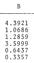
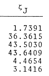
Corresponding Values Extracted Directly from [http://adsabs.harvard.edu/abs/1983PASAu...5..175M Murphy's (1983)] Table 3 | |||
</td> | |||
<td align="center" colspan="5"> | |||
| |||
</td> | |||
</tr> | |||
<tr> | |||
<td align="center">[[File:Table3CompleteCol1.png|center|50px|Column 1 from Table 3 of Murphy (1983)]]</td> | |||
<td align="right" colspan="2">[[File:Table3CompleteCol2.png|center|123px|Column 3 from Table 3 of Murphy (1983)]]</td> | |||
<td align="center"> </td> | |||
<td align="right">[[File:Table3CompleteCol3.png|center|67px|Column 3 from Table 3 of Murphy (1983)]]</td> | |||
<td align="right">[[File:Table3CompleteCol4.png|center|117px|Column 4 from Table 3 of Murphy (1983)]]</td> | |||
<td align="center"> </td> | |||
<td align="right">[[File:Table3CompleteCol5.png|center|71px|Column 5 from Table 3 of Murphy (1983)]]</td> | |||
<td align="right">[[File:Table3CompleteCol6.png|center|83px|Column 6 from Table 3 of Murphy (1983)]]</td> | |||
<td align="left" colspan="5">[[File:CommentButton02.png|left|100px|Comment by J. E. Tohline on 11 May 2015: | |||
The heading on this last column of numbers extracted from Murphy's (1983) paper has a subscript "J" whereas the subscript should be "R" to indicate the configuration's total radius.]]</td> | |||
</tr> | |||
<tr> | |||
<td align="left" colspan="14"> | |||
<sup>†</sup>See an [[User:Tohline/SSC/Structure/BiPolytropes/MurphyUVplane#Chandrasekhar.27s_U_and_V_Functions|accompanying discussion]] for definitions of the functions, <math>~U_{1E}</math>, <math>~V_{1E}</math>, <math>~U_{5F}</math>, and <math>~V_{5F} \, .</math> | |||
</td> | |||
</tr> | |||
</table> | </table> | ||
</div> | </div> | ||
Latest revision as of 21:38, 14 May 2015
UV Plane Functions as Analyzed by Murphy (1983)

|
|---|
| | Tiled Menu | Tables of Content | Banner Video | Tohline Home Page | |
This chapter supports and expands upon an accompanying discussion of the construction of a bipolytrope in which the core has an <math>~n_c=1</math> polytropic index and the envelope has an <math>~n_e=5</math> polytropic index. This system is particularly interesting because the entire structure can be described by closed-form, analytic expressions. Here we provide an in-depth analysis of the work published by J. O. Murphy (1983, Proc. Astr. Soc. of Australia, 5, 175) in which the derivation of this particular bipolytropic configuration was first attempted. As can be seen from the following list of "key references," however, this publication was only one of a series of interrelated works by Murphy. We will henceforth refer to this <math>~(n_c, n_e) = (1, 5)</math> system as "Murphy's bipolytrope."
Key References
- S. Srivastava (1968, ApJ, 136, 680) A New Solution of the Lane-Emden Equation of Index n = 5
- H. A. Buchdahl (1978, Australian Journal of Physics, 31, 115): Remark on the Polytrope of Index 5 — the result of this work by Buchdahl has been highlighted inside our discussion of bipolytropes with <math>~(n_c, n_e) = (5, 1)</math>.
- J. O. Murphy (1980a, Proc. Astr. Soc. of Australia, 4, 37): A Finite Radius Solution for the Polytrope Index 5
- J. O. Murphy (1980b, Proc. Astr. Soc. of Australia, 4, 41): On the F-Type and M-Type Solutions of the Lane-Emden Equation
- J. O. Murphy (1981, Proc. Astr. Soc. of Australia, 4, 205): Physical Characteristics of a Polytrope Index 5 with Finite Radius
- J. O. Murphy (1982, Proc. Astr. Soc. of Australia, 4, 376): A Sequence of E-Type Composite Analytical Solutions of the Lane-Emden Equation
- J. O. Murphy (1983, Australian Journal of Physics, 36, 453): Structure of a Sequence of Two-Zone Polytropic Stellar Models with Indices 0 and 1
- J. O. Murphy (1983, Proc. Astr. Soc. of Australia, 5, 175): Composite and Analytical Solutions of the Lane-Emden Equation with Polytropic Indices n = 1 and n = 5
- J. O. Murphy & R. Fiedler (1985a, Proc. Astr. Soc. of Australia, 6, 219): Physical Structure of a Sequence of Two-Zone Polytropic Stellar Models
- J. O. Murphy & R. Fiedler (1985b, Proc. Astr. Soc. of Australia, 6, 222): Radial Pulsations and Vibrational Stability of a Sequence of Two-Zone Polytropic Stellar Models
Relevant Lane-Emden Functions
As is detailed in our accompanying discussion, the Lane-Emden function governing the structure of the <math>~n_c = 1</math> core of Murphy's bipolytrope is,
<math> \theta(\xi) = \frac{\sin\xi}{\xi} \, , </math>
and the first derivative of this function with respect to the dimensionless radial coordinate, <math>~\xi</math>, is,
<math> \frac{d\theta}{d\xi} = -\frac{1}{\xi^{2}} (\sin\xi - \xi\cos\xi) \, . </math>
Also as is detailed in our accompanying discussion, the Lane-Emden function governing the structure of the <math>~n_e = 5</math> envelope of Murphy's bipolytrope is,
|
<math>~\phi(\xi)</math> |
<math>~=</math> |
<math>~\frac{B^{-1}\sin[\ln(A\xi)^{1/2})]}{\xi^{1/2}\{3-2\sin^2[\ln(A\xi)^{1/2}]\}^{1/2}} </math> |
|
|
<math>~=</math> |
<math>~\frac{B^{-1}\sin\Delta}{\xi^{1/2}(3-2\sin^2\Delta)^{1/2}} \, ,</math> |
and the first derivative of this function is,
|
<math>~\frac{d\phi}{d\xi}</math> |
<math>~=</math> |
<math>~- \frac{B^{-1}(3\sin\Delta - 2\sin^3\Delta -3\cos\Delta) }{2\xi^{3/2}(3-2\sin^2\Delta)^{3/2}} \, , </math> |
where we have adopted the shorthand notation,
<math>~\Delta \equiv \ln(A\xi)^{1/2} \, .</math>
Chandrasekhar's U and V Functions
As presented by Murphy (1983), most of the development and analysis of this model was conducted within the framework of what is commonly referred to in the astrophysics community as the "U-V" plane. Specifically in the context of the model's <math>~n_c=1</math> core, this pair of referenced functions is:
|
<math>~U_{1E} \equiv \xi \theta \biggl(- \frac{d\theta}{d\xi}\biggr)^{-1}</math> |
<math>~=</math> |
<math>~\sin\xi\biggl[\frac{1}{\xi^{2}} (\sin\xi - \xi\cos\xi)\biggr]^{-1}</math> |
|
|
<math>~=</math> |
<math>~\frac{\xi^2}{(1 - \xi\cot\xi)} \, ;</math> |
|
<math>~(n_c+1) V_{1E} \equiv (n_c+1)\frac{\xi}{ \theta} \biggl(- \frac{d\theta}{d\xi}\biggr)</math> |
<math>~=</math> |
<math>~\frac{2\xi^2}{\sin\xi} \biggl[ \frac{1}{\xi^{2}} (\sin\xi - \xi\cos\xi) \biggr]</math> |
|
|
<math>~=</math> |
<math>~ 2(1 - \xi\cot\xi) \, .</math> |
Correspondingly, in the context of the model's <math>~n_e=5</math> envelope, the pair of referenced functions is:
|
<math>~U_{5F} \equiv \xi \phi^5 \biggl(- \frac{d\phi}{d\xi}\biggr)^{-1}</math> |
<math>~=</math> |
<math>~ \frac{B^{-4}\xi \sin^5\Delta}{\xi^{5/2}\{3-2\sin^2\Delta\}^{5/2}} \biggl[ \frac{2\xi^{3/2}(3-2\sin^2\Delta)^{3/2}}{3\sin\Delta - 2\sin^3\Delta -3\cos\Delta } \biggr] </math> |
|
|
<math>~=</math> |
<math>~ \frac{2B^{-4}\sin^5\Delta}{[3-2\sin^2\Delta][3\sin\Delta - 2\sin^3\Delta -3\cos\Delta ]} </math> |
|
|
<math>~=</math> |
<math>~ \frac{-2B^{-4}\sin^5\Delta}{[2+\cos(2\Delta)][3\cos\Delta - \frac{3}{2}\sin\Delta - \frac{1}{2}\sin(3\Delta) ]} \, ; </math> |
|
<math>~(n_e+1) V_{5F} \equiv (n_e+1) \frac{\xi}{ \phi} \biggl(- \frac{d\phi}{d\xi}\biggr)</math> |
<math>~=</math> |
<math>~\frac{6\xi^{3/2}\{3-2\sin^2\Delta\}^{1/2}} {\sin\Delta} \frac{[3\sin\Delta - 2\sin^3\Delta -3\cos\Delta ] }{2\xi^{3/2}(3-2\sin^2\Delta)^{3/2}} </math> |
|
|
<math>~=</math> |
<math>~\frac{3[3\sin\Delta - 2\sin^3\Delta -3\cos\Delta ] }{\sin\Delta (3-2\sin^2\Delta)} </math> |
|
|
<math>~=</math> |
<math>~\frac{-6[3\cos\Delta - \frac{3}{2}\sin\Delta - \frac{1}{2}\sin(3\Delta) ] }{2\sin\Delta [2+\cos(2\Delta)]} \, . </math> |
In an effort to demonstrate correspondence with the published work of Murphy (1983), we have reproduced his expressions for these governing U-V functions in the following boxed-in image.
|
U-V Functions Extracted from Murphy (1983)
(slightly edited before reproduction as an image, here) |
The match between our expressions and those presented by Murphy becomes clear upon recognizing that, in our notation,
|
<math>~\Delta </math> |
<math>~=</math> |
<math>~\ln\sqrt{A\xi} </math> |
|
<math>~\Rightarrow ~~~~ 2\Delta </math> |
<math>~=</math> |
<math>~2 \ln\sqrt{A\xi} = \ln(A\xi) </math> |
|
and, <math>~3\Delta </math> |
<math>~=</math> |
<math>~3\ln[\sqrt{A\xi}] \, ;</math> |
and, in laying out these function definitions, Murphy has implicitly assumed that the two scaling coefficients, <math>~A</math> and <math>~B</math>, are unity.
CAUTION: Presented in this fashion — that is, by using <math>~\xi</math> to represent the dimensionless radial coordinate in all four expressions — Murphy's expressions seem to imply that the independent variable defining the radial coordinate in the bipolytrope's core is the same as the one that defines the radial coordinate in the structure's envelope. In general, this will not be the case, so we have explicitly used a different independent variable, <math>~\eta</math>, to mark the envelope's radial coordinate in our expressions. It is clear from other elements of his published derivation that Murphy understood this distinction but, as is explained more fully below, errors in his final model specifications may have resulted from not explicitly differentiating between this variable notation.
Critique of Murphy's Model Characteristics
Material that appears after this point in our presentation is under development and therefore
may contain incorrect mathematical equations and/or physical misinterpretations.
| Go Home |
As a supplement to the preceding two figures, the following table shows in quantitative detail how we are able to analytically derive individual coordinate roots, <math>~(A_0\eta)_\mathrm{root}</math> — see the next-to-last column of the table — from ten different interface-coordinate locations, <math>~\xi_i = \zeta_J</math>, as specified in the first (left-most) column of the table. The interface parameter, <math>~\kappa_i</math>, is determined directly from the specified value of <math>~\xi_i</math>; the parameter, <math>~p=(1-\kappa_i)^{-1}</math>; then, given <math>~p</math>, the root to the cubic equation and, in turn, the value of <math>~\Delta_i</math>, are determined; and, finally, a choice of the integer phase-shift parameter, <math>~m</math>, leads to the calculation of <math>~(A_0\eta)_\mathrm{root}</math>. For comparison, the last (right-most) column of the table lists the corresponding coordinate, <math>~\xi_J</math>, as originally derived and published by Murphy (1983). Coordinate pairs shown in the orange-colored panels of our table correspond to the six models whose characteristics are provided in Murphy's Table 3; coordinate pairs shown in the green-colored panels correspond to two of the ten "F2 = 0" roots identified in Murphy's Table 1; and the additional three coordinate pairs shown in the blue-colored panels have been drawn from Murphy's Table 2.
|
Murphy (1983) Tables 1, 2, & 3 |
Here … setting <math>\xi_i = \zeta_J</math> … and assuming <math>\mu_e/\mu_c = 1</math> |
Murphy (1983) Tables 1, 2, & 3 |
|||||
|
1st Constraint |
|||||||
|
<math>~\zeta_J</math> |
<math>~\kappa_i</math> |
<math>~p</math> |
<math>~y_\mathrm{root}</math> |
<math>~(\Delta_i-m\pi)</math><math>~= \tan^{-1}(y_\mathrm{root})</math> |
<math>~m </math> |
<math>~(A_0\eta)_\mathrm{root} = e^{2\Delta_i}</math> |
<math>~\xi_J</math> |
|
3.2678E-02 |
2.3732E-04 |
1.00023737 |
2.26083 |
1.15435 |
-3 |
6.55237E-08 |
6.55E-08 |
|
-2 |
3.50874E-05 |
3.508E-05 |
|||||
|
-1 |
1.87890E-02 |
1.8789E-02 |
|||||
|
0 |
10.0614 |
10.0164 |
|||||
|
0.8154 |
0.15474 |
1.18307 |
2.93939 |
1.24287 |
0 |
12.0101 |
12.0083 |
|
1.6598 |
0.76541 |
4.26281 |
12.6311 |
1.49179 |
0 |
19.7585 |
20.4312 |
|
[ 2.0914 ] |
1.46609 |
-2.14552 |
-6.11816 |
-1.40878 |
1 |
31.9964 |
33.0249 |
|
[ 2.10961 ] |
1.50744 |
-1.97067 |
-5.56379 |
-1.39296 |
1 |
33.0249 |
|
|
2.6914 |
4.37925 |
-0.29592 |
-0.31486 |
-0.30503 |
1 |
290.943 |
|
|
2.7302 |
4.83853 |
-0.26052 |
-0.27316 |
-0.26666 |
1 |
99.997<math>\pi</math> |
100<math>\pi</math> |
|
3.1415 |
22604.6 |
-4.42408E-05 |
-4.42408E-05 |
-4.42408E-05 |
2 |
91268<math>\pi</math> |
91275<math>\pi</math> |
|
4.2993 |
-0.58961 |
0.62908 |
0.89355 |
0.72924 |
0 |
4.2994 |
4.2993 |
|
7.6882 |
-0.19091 |
0.83969 |
1.6268 |
1.01964 |
0 |
7.6851 |
7.6882 |
As this table and the log-log plots presented in two preceding figures illustrate, by and large, the agreement between our analytically determined coordinate roots and those derived & published by Murphy (1983) is excellent. There are a couple of mismatches, but we attribute both to typesetting errors in the Murphy publication:
- The coordinate, <math>~\xi_J = 10.0164</math>, that has been displayed using a red font in the right-most column of our table is the value drawn directly from Murphy's Table 3. It appears to us that two digits of this number were inadvertently transposed during publication and that the coordinate value should have appeared as <math>~\xi_J = 10.0614</math>. We are convinced that, as published, this is a typographical error in Murphy's Table 3 because: (a) the corrected value matches our derived value of that coordinate to more significant figures, and (b) the same model is also listed in Murphy's Table 2 with this corrected value.
- The coordinate, <math>~\zeta_J = 2.6914</math>, that has been displayed using a red font in the left-most column of our table is the value drawn directly from Murphy's Table 3. As shown in our table, from this coordinate value we derive a root coordinate of <math>~(A_0\eta)_\mathrm{root} = 290.943</math>, which is almost a factor of ten larger than Murphy's published root coordinate value, <math>~\xi_J = 33.0249</math>. Working backwards via an iterative procedure, we have determined that Murphy's listed root of <math>33.0249</math> can be obtained if the originating value of <math>~\zeta_J \leftrightarrow \xi_i</math> is set to <math>2.10961</math> (see the black-on-white panel entry in the left-most column of our table). By replacing the "6" by a zero in Murphy's published coordinate parameter — that is, by assuming that there was a typographical error and Murphy's interface coordinate was actually <math>~\zeta_J = 2.0914</math>, we are able to derive a root coordinate value (31.9964) that is quite close to Murphy's published value (33.0249).
|
Model Characteristics from Murphy's Table 3 |
Implications |
||||||
|
Model |
<math>\xi = \zeta_J</math> |
<math>(A\xi) = \xi_J</math> |
<math>A = \xi_J/\zeta_J</math> |
<math>\Delta = \ln(A\xi)^{1/2}</math> |
<math>V_{1E}</math> |
<math>V_{5F}</math> |
<math>\frac{(n_c+1)V_{1E}}{(n_e+1)V_{5F}}</math> |
|
1 |
0.032678 |
10.0614 |
307.895 |
1.1544 |
3.5598E-04 |
1.1871E-04 |
1.000 |
|
2 |
0.8154 |
12.0083 |
14.727 |
1.2428 |
2.3212E-01 |
7.7302E-02 |
1.001 |
|
3 |
1.6598 |
20.4312 |
12.309 |
1.5085 |
1.1481 |
0.40720 |
0.940 |
|
4 |
2.6914 |
33.0249 |
12.2704 |
1.7486 |
6.5689 |
0.75371 |
2.905 |
|
5 |
2.7302 |
314.159 |
115.068 |
2.8750 |
7.2578 |
2.4193 |
1.000 |
|
6 |
3.1415 |
2.8675E+05 |
9.1278E+04 |
6.2832 |
3.3907E+04 |
2.9313E+04 |
0.386 |
|
NOTE: As is explained in an accompanying discussion, we suspect that the two numbers drawn from Murphy's Table 3 that are displayed here in a red font contain typographical errors. |
|||||||
|
Some Model Characteristics (assuming <math>\mu_e/\mu_c</math> = 1) |
|||||||||||||
|
Model |
Specified |
Analytically Determined Here |
… and Constraint Implications† |
||||||||||
|
<math>~\xi_i</math> |
<math>~m</math> |
<math>~\Delta_i</math> |
<math>~(A_0\eta)_\mathrm{root}</math> |
<math>~\frac{A_0}{3^{1/2}} \biggl( \frac{\mu_e}{\mu_c} \biggr) </math> |
<math>~B_0</math> |
<math>~\frac{B_0}{3^{1/4}} \biggl(\frac{\mu_e}{\mu_c}\biggr)^{1/2} \theta_i^{-1} </math> |
<math>~\xi_s</math> |
<math>~V_{1E}</math> |
<math>~V_{5F}</math> |
<math>\frac{(n_c+1)V_{1E}}{(n_e+1)V_{5F}}</math> |
<math>~U_{1E}</math> |
<math>\frac{U_{1E}}{U_{5F}}</math> |
|
| 1 | 3.2678E-02 | 0 | 1.1544 | 10.0614 | 307.894 | 5.77929 | 4.39209 | 1.7392 | 3.5598E-04 | 1.1866E-4 | 1.000 | 2.9998 | 1.000 |
| 2 | 0.8154 | 0 | 1.2429 | 12.0101 | 14.729 | 1.25567 | 1.06865 | 36.356 | 0.23212 | 0.077372 | 1.000 | 2.8644 | 1.000 |
| 3 | 1.6598 | 0 | 1.4918 | 19.7585 | 11.9041 | 1.01206 | 1.28146 | 44.984 | 1.14812 | 0.38271 | 1.000 | 2.3995 | 1.000 |
| 4 | 2.0914 | 1 | 1.7328 | 31.9964 | 15.2990 | 0.87563 | 1.60398 | 35.0016 | 2.19913 | 0.73304 | 1.000 | 1.98894 | 1.000 |
| 5 | 2.7302 | 1 | 2.8749 | 100.00<math>\pi</math> | 115.065 | 0.12408 | 0.64370 | 4.6539 | 7.25779 | 2.41926 | 1.000 | 1.02703 | 1.000 |
| 6 | 3.1415 | 2 | 6.283141 | 91268<math>\pi</math> | 170.44223<math>e^{2\pi}</math> | 1.8966E-05 | 0.48862 | 3.141778 | 3.3907E+04 | 1.1302E+04 | 1.000 | 2.9106E-04 | 1.000 |
|
Corresponding Values Extracted Directly from Murphy's (1983) Table 3 |
|
||||||||||||
|
†See an accompanying discussion for definitions of the functions, <math>~U_{1E}</math>, <math>~V_{1E}</math>, <math>~U_{5F}</math>, and <math>~V_{5F} \, .</math> |
|||||||||||||
Related Discussions

|
|---|
|
© 2014 - 2021 by Joel E. Tohline |


