User:Tohline/SSC/Stability/MurphyFiedler85

Review of the BiPolytrope Stability Analysis by Murphy & Fiedler (1985b)

Overview

In the stability analysis presented by Murphy & Fiedler (1985b), the relevant polytropic indexes are, <math>~(n_c, n_e) = (1,5)</math>. Structural properties of the underlying equilibrium models have been reviewed in our accompanying discussion.

The Linear Adiabatic Wave Equation (LAWE) that is relevant to polytropic spheres may be written as,

	<math>~0 = \frac{d^2x}{d\xi^2} + \biggl[ 4 - (n+1) Q \biggr] \frac{1}{\xi} \cdot \frac{dx}{d\xi} + (n+1) \biggl[ \biggl( \frac{\sigma_c^2}{6\gamma_g } \biggr) \frac{\xi^2}{\theta} - \alpha Q\biggr] \frac{x}{\xi^2} </math>
where:    <math>~Q(\xi) \equiv - \frac{d\ln\theta}{d\ln\xi} \, ,</math>    <math>~\sigma_c^2 \equiv \frac{3\omega^2}{2\pi G\rho_c} \, ,</math>     and,     <math>~\alpha \equiv \biggl(3 - \frac{4}{\gamma_\mathrm{g}}\biggr)</math>

See also … Accompanying chapter showing derivation and overlap with multiple classic papers: A. S. Eddington (1926), especially equation (127.6) on p. 188 — The Internal Constitution of Stars P. Ledoux & C. L. Pekeris (1941, ApJ, 94, 124) — Radial Pulsations of Stars M. Schwarzschild (1941, ApJ, 94, 245) — Overtone Pulsations for the Standard Model R. F. Christy (1966, Annual Reviews of Astronomy & Astrophysics, 4, 353) — Pulsation Theory J. P. Cox (1974, Reports on Progress in Physics, 37, 563) — Pulsating Stars Accompanying chapter detailing specific application to polytropes along with a couple of additional key references: M. Hurley, P. H. Roberts, & K. Wright (1966, ApJ, 143, 535) — The Oscillations of Gas Spheres Murphy & Fiedler (1985b) — Radial Pulsations and Vibrational Stability of a Sequence of Two Zone Polytropic Stellar Models

As we have detailed separately, the boundary condition at the center of a polytropic configuration is,

<math>~\frac{dx}{d\xi} \biggr|_{\xi=0} = 0 \, ;</math>

and the boundary condition at the surface of an isolated polytropic configuration is,

<math>~\frac{d\ln x}{d\ln\xi}</math>

<math>~=</math>

<math>~- \alpha + \frac{\omega^2}{\gamma_g } \biggl( \frac{1}{4\pi G \rho_c } \biggr) \frac{\xi}{(-\theta^')} </math>         at         <math>~\xi = \xi_s \, .</math>

Murphy & Fiedler (1985b) apparently decided that they could not simply integrate the above-presented polytropic LAWE from the center of the configuration to its surface because the underlying bipolytropic equilibrium structure of the envelope and the core are defined by two different polytropic indexes. Instead, they separated the problem into two pieces — integrating the relevant core LAWE from the center to the core-envelope interface, then integrating the relevant envelope LAWE from that interface to the surface — being careful to properly match the two solutions at the interface.

They also realized that the above-specified surface boundary condition is not applicable to bipolytropes. Instead, they used what we will refer to as the original, more general expression of the surface boundary condition:

<math>~ \frac{d\ln x}{d\ln\xi}\biggr|_s</math>

<math>~=</math>

<math>~- \alpha + \frac{\omega^2 R^3}{\gamma_g GM_\mathrm{tot}} \, .</math>

Utilizing an accompanying discussion, let's examine the frequency normalization used by Murphy & Fiedler (1985b) (see the top of the left-hand column on p. 223): <math>~\Omega^2</math> <math>~\equiv</math> <math>~ \omega^2 \biggl[ \frac{R^3}{GM_\mathrm{tot}} \biggr] </math>   <math>~=</math> <math>~ \omega^2 \biggl[ \frac{3}{4\pi G \bar\rho} \biggr] = \omega^2 \biggl[ \frac{3}{4\pi G \rho_c} \biggr] \frac{\rho_c}{\bar\rho} = \frac{3\omega^2}{(n_c+1)} \biggl[ \frac{(n_c+1)}{4\pi G \rho_c} \biggr] \frac{\rho_c}{\bar\rho} </math>   <math>~=</math> <math>~ \frac{3\omega^2}{(n_c+1)} \biggl[ \frac{a_n^2\rho_c}{P_c} \cdot \theta_c \biggr] \frac{\rho_c}{\bar\rho} = \frac{3\gamma}{(n_c+1)} \frac{\rho_c}{\bar\rho} \biggl[ \frac{a_n^2\rho_c}{P_c} \cdot \frac{\omega^2 \theta_c}{\gamma} \biggr] \, . </math> For a given radial quantum number, <math>~k</math>, the factor inside the square brackets in this last expression is what Murphy & Fiedler (1985b) refer to as <math>~\omega^2_k \theta_c</math>. Keep in mind, as well, that, in the notation we are using, <math>~\sigma_c^2</math> <math>~\equiv</math> <math>~\frac{3\omega^2}{2\pi G \rho_c}</math> <math>~\Rightarrow ~~~ \sigma_c^2</math> <math>~=</math> <math>~ \biggl( \frac{2\bar\rho}{\rho_c}\biggr) \Omega^2 = \frac{6\gamma}{(n_c+1)} \biggl[ \frac{a_n^2\rho_c}{P_c} \cdot \frac{\omega^2 \theta_c}{\gamma} \biggr] = \frac{6\gamma}{(n_c+1)} \biggl[ \omega_k^2 \theta_c \biggr] \, . </math> This also means that the surface boundary condition may be rewritten as, <math>~ \frac{d\ln x}{d\ln\xi}\biggr|_s</math> <math>~=</math> <math>~\frac{\Omega^2}{\gamma_g } - \alpha \, .</math>

Aside Regarding Convectively Unstable Core

It is worth highlighting that, in their effort to determine the eigenvectors associated with radial pulsations in <math>~(n_c, n_e) = (1, 5)</math> bipolytropes, Murphy & Fiedler (1985b) assumed that fluid elements throughout the entire spherical configuration expand and contract along <math>~\gamma_g = 5/3</math> adiabats. Referencing separately the structural polytropic index of the core and of the envelope of the equilibrium bipolytropic models, we see that,

<math>~\gamma_g</math>

<math>~< </math>

<math>~\frac{n_c+1}{n_c} = 2 \, ,</math>

while,

<math>~\gamma_g</math>

<math>~></math>

<math>~\frac{n_e+1}{n_e} = \frac{6}{5} \, .</math>

According to the so-called Schwarzschild criterion — see, for example, our accompanying discussion titled, Axisymmetric Instabilities to Avoid — it therefore seems that the core of each of their equilibrium models should have been convectively unstable. Murphy & Fiedler (1985b) did not comment on the impact that the presence of a convective core should have had on their radial pulsation analysis.

More Detailed Setup

Here we describe in more detail the steps that Murphy & Fiedler (1985b) employed in order to numerically determine the radial-oscillation eigenvectors of <math>~(n_c, n_e) = (1, 5)</math> bipolytropic spheres.

Core Layers With n = 1

For n = 1 structures the LAWE is,

<math>~0</math>

<math>~=</math>

<math>~ \frac{d^2x}{d\xi^2} + \biggl[ 4 - 2 Q_1 \biggr] \frac{1}{\xi} \cdot \frac{dx}{d\xi} + 2 \biggl[ \biggl( \frac{\sigma_c^2}{6\gamma_\mathrm{core} } \biggr) \frac{\xi^2}{\theta} - \alpha_\mathrm{core} Q_1\biggr] \frac{x}{\xi^2} </math>

where,

<math>~Q_1</math>

<math>~\equiv</math>

<math>~- \frac{d\ln\theta}{d\ln\xi} \, .</math>

Given that, for <math>~n = 1</math> polytropic structures,

<math> \theta(\xi) = \frac{\sin\xi}{\xi} </math>       and       <math> \frac{d\theta}{d\xi} = \biggl[ \frac{\cos\xi}{\xi}- \frac{\sin\xi}{\xi^2}\biggr] </math>

we have,

<math>~Q_1</math>	<math>~=</math>	<math>~ - \frac{\xi^2}{\sin\xi} \biggl[ \frac{\cos\xi}{\xi}- \frac{\sin\xi}{\xi^2}\biggr] </math>
	<math>~=</math>	<math>~ 1 - \xi\cot\xi \, . </math>

Hence, the governing LAWE for the core is,

<math>~0</math>	<math>~=</math>	<math>~ \frac{d^2x}{d\xi^2} + \biggl[ 4 - 2 ( 1 - \xi\cot\xi ) \biggr] \frac{1}{\xi} \cdot \frac{dx}{d\xi} + 2 \biggl[ \biggl( \frac{\sigma_c^2}{6\gamma_\mathrm{core} } \biggr) \frac{\xi^3}{\sin\xi} - \alpha_\mathrm{core} ( 1 - \xi\cot\xi )\biggr] \frac{x}{\xi^2} </math>
	<math>~=</math>	<math>~ \frac{d^2x}{d\xi^2} + \biggl[ 1 + \xi\cot\xi \biggr] \frac{2}{\xi} \cdot \frac{dx}{d\xi} + 2 \biggl[ \biggl( \frac{\sigma_c^2}{6\gamma_\mathrm{core} } \biggr) \frac{\xi^3}{\sin\xi} - \alpha_\mathrm{core} ( 1 - \xi\cot\xi )\biggr] \frac{x}{\xi^2} \, . </math>

This can be rewritten as,

<math>~0</math>	<math>~=</math>	<math>~ \frac{d^2x}{d\xi^2} + \frac{2}{\xi} \biggl[ 1 + \xi\cot\xi \biggr]\frac{dx}{d\xi} + \biggl[ \biggl( \frac{\sigma_c^2}{3\gamma_\mathrm{core} } \biggr) \frac{\xi}{\sin\xi} + \frac{2 \alpha_\mathrm{core} ( \xi\cos\xi - \sin\xi) }{\xi^2 \sin\xi} \biggr] x </math>
	<math>~=</math>	<math>~ \frac{d^2x}{d\xi^2} + \frac{2}{\xi} \biggl[ 1 + \xi\cot\xi \biggr]\frac{dx}{d\xi} + \biggl[ \frac{\gamma_g}{\gamma_\mathrm{core}}\biggl( \omega_k^2 \theta_c \biggr) \frac{\xi}{\sin\xi} + \frac{2 \alpha_\mathrm{core} ( \xi\cos\xi - \sin\xi) }{\xi^2 \sin\xi} \biggr] x \, , </math>

which matches the expression presented by Murphy & Fiedler (1985b) (see middle of the left column on p. 223 of their article) if we set <math>~\theta_c = 1</math> and <math>~\gamma_g/\gamma_\mathrm{core} = 1</math>. This LAWE also appears in our separate discussion of radial oscillations in n = 1 polytropic spheres.

Envelope Layers With n = 5

The LAWE for n = 5 structures is,

<math>~0</math>

<math>~=</math>

<math>~ \frac{d^2x}{d\eta^2} + \biggl[ 4 - 6Q_5 \biggr] \frac{1}{\eta} \cdot \frac{dx}{d\eta} + 6 \biggl[ \biggl( \frac{\sigma_c^2}{6\gamma_\mathrm{env} } \biggr) \frac{\eta^2}{\phi} - \alpha_\mathrm{env} Q_5\biggr] \frac{x}{\eta^2} </math>

where,

<math>~Q_5</math>

<math>~\equiv</math>

<math>~- \frac{d\ln\phi}{d\ln\eta} \, .</math>

From our accompanying discussion of the underlying equilibrium structure of <math>~(n_c, n_e) = (1, 5)</math> bipolytropes, we know that,

<math>~\phi</math>

<math>~=</math>

<math>~\frac{B_0^{-1}\sin\Delta}{\eta^{1/2}(3-2\sin^2\Delta)^{1/2}} \, ,</math>

and,

<math>~\frac{d\phi}{d\eta}</math>

<math>~=</math>

<math>~ \frac{B_0^{-1}[3\cos\Delta-3\sin\Delta + 2\sin^3\Delta] }{2\eta^{3/2}(3-2\sin^2\Delta)^{3/2}} \, . </math>

where <math>~A_0</math> is a "homology factor," <math>~B_0</math> is an overall scaling coefficient, and we have introduced the notation,

<math>~\Delta \equiv \ln(A_0\eta)^{1/2} = \frac{1}{2} (\ln A_0 + \ln\eta) \, .</math>

Hence,

<math>~Q_5</math>	<math>~=</math>	<math>~ - \eta \biggl[ \frac{\eta^{1/2}(3-2\sin^2\Delta)^{1/2}}{B_0^{-1}\sin\Delta} \biggr] \frac{B_0^{-1}[3\cos\Delta-3\sin\Delta + 2\sin^3\Delta] }{2\eta^{3/2}(3-2\sin^2\Delta)^{3/2}} </math>
	<math>~=</math>	<math>~ \frac{ 3\sin\Delta - 3\cos\Delta - 2\sin^3\Delta }{2 \sin\Delta (3-2\sin^2\Delta)} \, . </math>

And,

<math>~0</math>	<math>~=</math>	<math>~ \frac{d^2x}{d\eta^2} ~+~ \biggl[ 4 + \frac{ 3(3\cos\Delta - 3\sin\Delta + 2\sin^3\Delta) }{ \sin\Delta (3-2\sin^2\Delta)} \biggr] \frac{1}{\eta} \cdot \frac{dx}{d\eta} ~+~ \biggl[ \biggl( \frac{\sigma_c^2}{\gamma_\mathrm{env} } \biggr) \frac{B_0 \eta^{1/2}(3-2\sin^2\Delta)^{1/2}}{\sin\Delta} ~+~ \frac{ 3\alpha_\mathrm{env} (3\cos\Delta -3\sin\Delta + 2\sin^3\Delta )}{\eta^2 \sin\Delta (3-2\sin^2\Delta)}\biggr] x </math>
	<math>~=</math>	<math>~ \frac{d^2x}{d\eta^2} ~+~ \biggl[ 4 ~+~ \frac{ 3(3\cos\Delta - \tfrac{3}{2}\sin\Delta - \tfrac{1}{2}\sin3\Delta) }{ \sin\Delta (2 + \cos2\Delta)} \biggr] \frac{1}{\eta} \cdot \frac{dx}{d\eta} ~+~ \biggl[\omega^2_k \theta_c \biggl( \frac{\gamma_g}{\gamma_\mathrm{env} } \biggr) \frac{B_0 \eta^{1/2}(2 + \cos2\Delta)^{1/2}}{\sin\Delta} ~+~ \frac{ 3\alpha_\mathrm{env} (3\cos\Delta -\tfrac{3}{2}\sin\Delta - \tfrac{1}{2}\sin3\Delta )}{\eta^2 \sin\Delta (2 + \cos2\Delta)}\biggr] x \, , </math>

which matches the expression presented by Murphy & Fiedler (1985b) (see middle of the left column on p. 223 of their article) if we set <math>~\theta_c = 1</math> and <math>~\gamma_g/\gamma_\mathrm{env} = 1</math>.

Surface Boundary Condition

Next, pulling from our accompanying discussion of the stability of polytropes and an accompanying table that details the properties of <math>~(n_c, n_e) = (1, 5)</math> bipolytropes, the surface boundary condition is,

<math>~ \frac{d\ln x}{d\ln\eta}\biggr|_s</math>	<math>~=</math>	<math>~- \biggl(\frac{\gamma_g}{\gamma_\mathrm{env}}\biggr) \alpha + \frac{\omega^2 R^3}{\gamma_\mathrm{env} GM_\mathrm{tot}} </math>
<math>~\Rightarrow ~~~ \frac{d\ln x}{d\ln\eta}\biggr|_s + \biggl(\frac{\gamma_g}{\gamma_\mathrm{env}}\biggr) \alpha </math>	<math>~=</math>	<math>~ \frac{\omega^2 (R_s^*)^3}{\gamma_\mathrm{env} GM^*_\mathrm{tot}} \biggl( \frac{K_c}{G}\biggr)^{3 / 2}\biggl( \frac{K_c}{G}\biggr)^{-3 / 2} \frac{1}{\rho_0}</math>
	<math>~=</math>	<math>~ \frac{\omega^2 }{\gamma_\mathrm{env} G\rho_0 } \biggl[ (2\pi)^{-1/2} \xi_i e^{2(\pi - \Delta_i)} \biggr]^3 \biggl[ \biggl( \frac{3}{2\pi} \biggr)^{1/2} \sin\xi_i \biggl( \frac{3}{\sin^2\Delta_i} - 2 \biggr)^{1/2} e^{(\pi - \Delta_i)} \biggr]^{-1} \biggl( \frac{\mu_e}{\mu_c}\biggr)</math>
	<math>~=</math>	<math>~ \frac{\omega^2 }{\gamma_\mathrm{env}(2\pi G\rho_0)} \biggl( \frac{\mu_e}{\mu_c}\biggr) \frac{1}{\sqrt{3}} \biggl[ \frac{\xi_i^2}{\theta_i} \biggr] \biggl( \frac{3}{\sin^2\Delta_i} - 2 \biggr)^{-1 / 2} e^{5(\pi - \Delta_i)}</math>
	<math>~=</math>	<math>~ \frac{\omega^2 }{\gamma_\mathrm{env}(2\pi G\rho_0)} \biggl( \frac{\mu_e}{\mu_c}\biggr) \frac{e^{5\pi}}{\sqrt{3}} \biggl[ \frac{\xi_i^2}{\theta_i} \biggr] \xi_i^{1 / 2}B\theta_i (\xi_i A)^{-5/2}</math>
	<math>~=</math>	<math>~ \frac{\omega^2 }{\gamma_\mathrm{env}(2\pi G\rho_0)} \biggl( \frac{\mu_e}{\mu_c}\biggr) \frac{B e^{5\pi}}{\sqrt{3} ~A^{5 / 2}} </math>
	<math>~=</math>	<math>~ \frac{2\omega_k^2 \theta_c}{(n_c+1)} \biggl( \frac{\mu_e}{\mu_c}\biggr) \frac{B e^{5\pi}}{\sqrt{3} ~A^{5 / 2}} \, . </math>

After acknowledging that, in their specific stability analysis, <math>~\theta_c = 1</math>, <math>~n_c = 1</math>, and <math>~\mu_e/\mu_c = 1</math>, this right-hand-side expression matches the equivalent term published by Murphy & Fiedler (1985b) (see the bottom of the left-hand column on p. 223).

Interface Conditions

Here, we will simply copy the discussion already provided in the context of our attempt to analyze the stability of <math>~(n_c, n_e) = (0, 0)</math> bipolytropes; specifically, we will draw from STEP 4: in the Piecing Together subsection. Following the discussion in §§57 & 58 of P. Ledoux & Th. Walraven (1958), the proper treatment is to ensure that fractional perturbation in the gas pressure (see their equation 57.31),

<math>~\frac{\delta P}{P}</math>

<math>~=</math>

<math>~- \gamma x \biggl( 3 + \frac{d\ln x}{d\ln \xi} \biggr) \, ,</math>

is continuous across the interface. That is to say, at the interface <math>~(\xi = \xi_i)</math>, we need to enforce the relation,

<math>~0</math>	<math>~=</math>	<math>~\biggl[ \gamma_c x_\mathrm{core} \biggl( 3 + \frac{d\ln x_\mathrm{core}}{d\ln \xi} \biggr) - \gamma_e x_\mathrm{env} \biggl( 3 + \frac{d\ln x_\mathrm{env}}{d\ln \xi} \biggr)\biggr]_{\xi=\xi_i}</math>
	<math>~=</math>	<math>~\gamma_e \biggl[ \frac{\gamma_c}{\gamma_e} \biggl( 3 + \frac{d\ln x_\mathrm{core}}{d\ln \xi} \biggr) - \biggl( 3 + \frac{d\ln x_\mathrm{env}}{d\ln \xi} \biggr)\biggr]_{\xi=\xi_i}</math>
<math>~\Rightarrow~~~ \frac{d\ln x_\mathrm{env}}{d\ln \xi} \biggr|_{\xi=\xi_i}</math>	<math>~=</math>	<math>~3\biggl(\frac{\gamma_c}{\gamma_e} -1\biggr) + \frac{\gamma_c}{\gamma_e} \biggl( \frac{d\ln x_\mathrm{core}}{d\ln \xi} \biggr)_{\xi=\xi_i} \, .</math>

In the context of this interface-matching constraint (see their equation 62.1), P. Ledoux & Th. Walraven (1958) state the following:   In the static (i.e., unperturbed equilibrium) model … discontinuities in <math>~\rho</math> or in <math>~\gamma</math> might occur at some [radius]. In the first case — that is, a discontinuity only in density, while <math>~\gamma_e = \gamma_c</math> — the interface conditions imply the continuity of <math>~\tfrac{1}{x} \cdot \tfrac{dx}{d\xi}</math> at that [radius]. In the second case — that is, a discontinuity in the adiabatic exponent — the dynamical condition may be written as above. This implies a discontinuity of the first derivative at any discontinuity of <math>~\gamma</math>.

The algorithm that Murphy & Fiedler (1985b) used to "… [integrate] through each zone …" was designed "… with continuity in <math>~x</math> and <math>~dx/d\xi</math> being imposed at the interface …" Given that they set <math>~\gamma_c = \gamma_e = 5/3</math>, their interface matching condition is consistent with the one prescribed by P. Ledoux & Th. Walraven (1958).

Our Confession

When we tried to integrate the governing LAWEs in the piecemeal fashion described by Murphy & Fiedler (1985b) — as we have just detailed — we initially failed to match their published eigenvector solutions. In retrospect, it appears as though we did not correctly implement the interface-matching conditions. In an effort to diagnose this problem, we backed up to a more generalized prescription of the LAWE that allowed us to smoothly integrate a single equation from the center to the surface of the configuration without having to mess with interface-matching conditions. In what follows, we describe this alternate approach. This approach has allowed us to derive radial-oscillation eigenvectors that match in detail the results published by Murphy & Fiedler (1985b).

An Alternate Approach

In an accompanying discussion, we derived the so-called,

Linear Adiabatic Wave (or Radial Pulsation) Equation

<math>~ \frac{d^2x}{dr_0^2} + \biggl[\frac{4}{r_0} - \biggl(\frac{g_0 \rho_0}{P_0}\biggr) \biggr] \frac{dx}{dr_0} + \biggl(\frac{\rho_0}{\gamma_\mathrm{g} P_0} \biggr)\biggl[\omega^2 + (4 - 3\gamma_\mathrm{g})\frac{g_0}{r_0} \biggr] x = 0 </math>

whose solution identifies eigenvectors that describe various radial modes of oscillation in spherically symmetric, self-gravitating fluid configurations. In shifting from this more general LAWE expression to the so-called polytropic LAWE — as presented above — the functions that quantify the structure of the underlying equilibrium configuration, <math>~\rho_0(r_0)</math>, <math>~P_0(r_0)</math>, and <math>~g_0(r_0)</math>, are re-expressed in terms of the polytropic function, <math>~\theta(\xi)</math> [or, instead, Φ(η)] and its derivative, and the dimensional Lagrangian radial coordinate, <math>~r_0</math>, is abandoned in favor the dimensionless Lagrangian radial coordinate, <math>~\xi</math> (or, instead, η), that is familiarly associated with a chosen polytropic index. In order to avoid confusion that might be associated with switching from one polytropic function to another at the core-envelope interface, here we have chosen to stick with the single Lagrangian radial coordinate, <math>~r_0</math>, throughout the configuration.

Foundation

Assuming that the underlying equilibrium structure is that of a bipolytrope having <math>~(n_c, n_e) = (1, 5)</math>, it makes sense to adopt the normalizations used when defining the equilibrium structure, namely,

<math>~\rho^*</math>	<math>~\equiv</math>	<math>~\frac{\rho_0}{\rho_c}</math>	;	<math>~r^*</math>	<math>~\equiv</math>	<math>~\frac{r_0}{(K_c/G)^{1/2}}</math>
<math>~P^*</math>	<math>~\equiv</math>	<math>~\frac{P_0}{K_c\rho_c^{2}}</math>	;	<math>~M_r^*</math>	<math>~\equiv</math>	<math>~\frac{M(r_0)}{\rho_c (K_c/G)^{3/2}}</math>
<math>~H^*</math>	<math>~\equiv</math>	<math>~\frac{H}{K_c\rho_c}</math>	.

We note as well that,

<math>~g_0</math>	<math>~=</math>	<math>~\frac{GM(r_0)}{r_0^2}</math>
	<math>~=</math>	<math>~ G \biggl[ M_r^* \rho_c \biggl( \frac{K_c}{G}\biggr)^{3 / 2} \biggr] \biggl[ r^*\biggl( \frac{K_c}{G}\biggr)^{1 / 2} \biggr]^{-2} </math>
	<math>~=</math>	<math>~ \frac{ M_r^*}{(r^*)^2}\biggl[ G\rho_c \biggl( \frac{K_c}{G}\biggr)^{1 / 2} \biggr] \, . </math>

Hence, multiplying the LAWE through by <math>~(K_c/G)</math> gives,

<math>~0</math>	<math>~=</math>	<math>~ \frac{d^2x}{dr*^2} + \biggl[\frac{4}{r^*} -\biggl( \frac{K_c}{G} \biggr)^{1 / 2}\biggl(\frac{g_0 \rho_0}{P_0}\biggr) \biggr] \frac{dx}{dr*} + \biggl( \frac{K_c}{G} \biggr)\biggl(\frac{\rho_0}{\gamma_\mathrm{g} P_0} \biggr)\biggl[\omega^2 + (4 - 3\gamma_\mathrm{g})\frac{g_0}{r_0} \biggr] x </math>
	<math>~=</math>	<math>~ \frac{d^2x}{dr*^2} + \biggl\{ \frac{4}{r^*} -\biggl( \frac{K_c}{G} \biggr)^{1 / 2}\biggl(\frac{\rho_c \rho^*}{P^* K_c \rho_c^2}\biggr)\frac{ M_r^*}{(r^*)^2}\biggl[ G\rho_c \biggl( \frac{K_c}{G}\biggr)^{1 / 2} \biggr] \biggr\} \frac{dx}{dr*} + \biggl( \frac{K_c}{G} \biggr)\biggl(\frac{\rho^*\rho_c}{\gamma_\mathrm{g} P^* K_c \rho_c^2} \biggr)\biggl\{ \omega^2 + (4 - 3\gamma_\mathrm{g})\frac{1}{r^*} \biggl(\frac{G}{K_c}\biggr)^{1 / 2}\frac{ M_r^*}{(r^*)^2}\biggl[ G\rho_c \biggl( \frac{K_c}{G}\biggr)^{1 / 2} \biggr]\biggr\} x </math>
	<math>~=</math>	<math>~ \frac{d^2x}{dr*^2} + \biggl\{ \frac{4}{r^*} -\biggl(\frac{\rho^*}{P^*}\biggr)\frac{ M_r^*}{(r^*)^2}\biggr\} \frac{dx}{dr*} + \biggl( \frac{1}{\gamma_\mathrm{g}G\rho_c} \biggr)\biggl(\frac{\rho^*}{ P^* } \biggr)\biggl\{ \omega^2 + (4 - 3\gamma_\mathrm{g})\frac{1}{r^*} \frac{ M_r^*}{(r^*)^2}\biggl[ G\rho_c \biggr]\biggr\} x </math>
	<math>~=</math>	<math>~ \frac{d^2x}{dr*^2} + \biggl\{ \frac{4}{r^*} -\biggl(\frac{\rho^*}{P^*}\biggr)\frac{ M_r^*}{(r^*)^2}\biggr\} \frac{dx}{dr*} + \biggl(\frac{\rho^*}{ P^* } \biggr)\biggl\{ \frac{\omega^2}{\gamma_\mathrm{g} G\rho_c} + \biggl(\frac{4}{\gamma_\mathrm{g}} - 3\biggr)\frac{1}{r^*} \frac{ M_r^*}{(r^*)^2}\biggr\} x </math>
	<math>~=</math>	<math>~ \frac{d^2x}{dr*^2} + \biggl\{ 4 -\biggl(\frac{\rho^*}{P^*}\biggr)\frac{ M_r^*}{(r^*)}\biggr\}\frac{1}{r^*} \frac{dx}{dr*} + \biggl(\frac{\rho^*}{ P^* } \biggr)\biggl\{ \frac{2\pi \sigma_c^2}{3\gamma_\mathrm{g}} ~-~\frac{\alpha_\mathrm{g} M_r^*}{(r^*)^3}\biggr\} x \, . </math>

This is the form of the LAWE that we will integrate from the center of the configuration to its surface <math>~(r^* = R^*)</math> in order to identify various eigenvectors that are associated with radial oscillations in <math>~(n_c, n_e) = (1, 5)</math> bipolytropes. Before performing the numerical integrations, we need only specify the underlying dimensionless structural functions, <math>~\rho^*(r^*)</math>, <math>~P^*(r^*)</math>, and <math>~M_r^*(r^*)</math>, throughout the underlying equilibrium configuration.

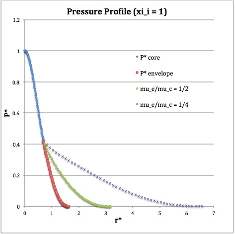
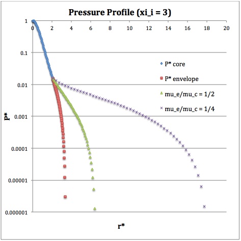
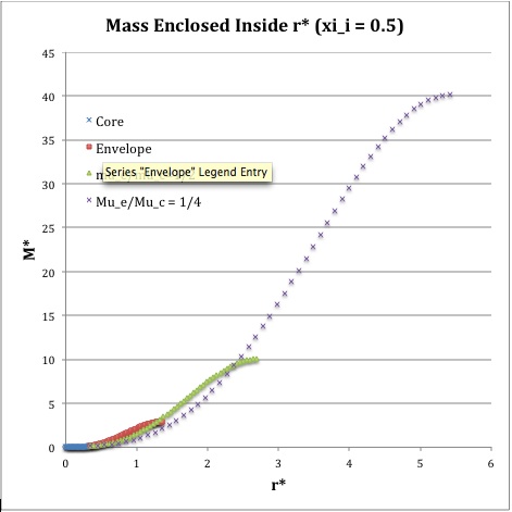
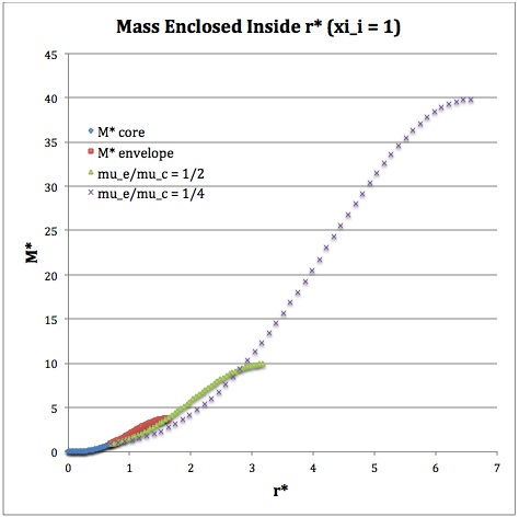
Profile

Referencing the relevant derived bipolytropic model profile, we should incorporate the following relations:

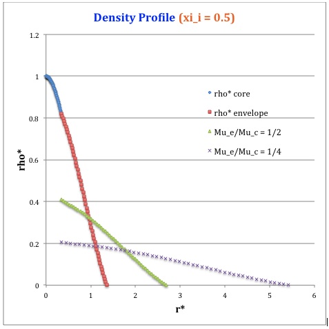
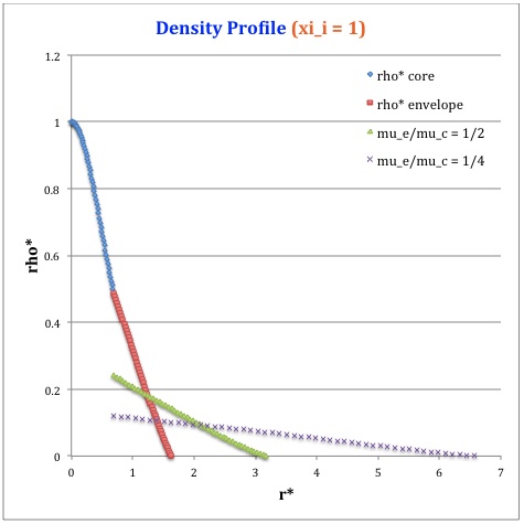
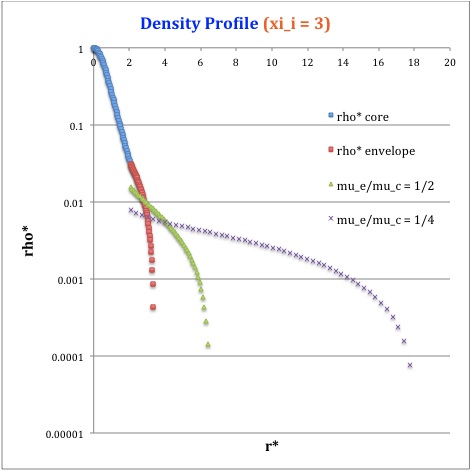
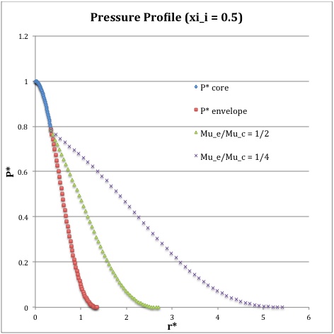
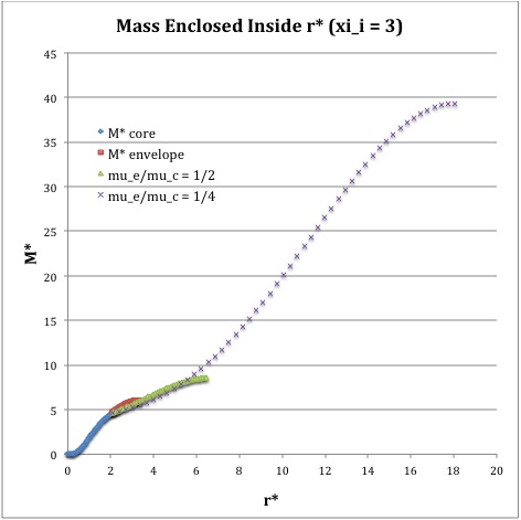
Variable	Throughout the Core <math>0 \le r^* \le \frac{\xi_i}{\sqrt{2\pi}}</math>	Throughout the Envelope† <math>\frac{\xi_i}{\sqrt{2\pi}} \le r^* \le \frac{\xi_i e^{2(\pi - \Delta_i)}}{\sqrt{2\pi}}</math>	Plotted Profiles
			<math>\xi_i = 0.5</math>	<math>\xi_i = 1.0</math>	<math>\xi_i = 3.0</math>
	<math>\xi = \sqrt{2\pi}~r^*</math>	<math>\eta = \biggl( \frac{\mu_e}{\mu_c} \biggr) \biggl(\frac{2\pi}{3}\biggr)^{1 / 2}~r^*</math>
<math>~\rho^*</math>	<math>\frac{\sin\xi}{\xi}</math>	<math>\biggl( \frac{\mu_e}{\mu_c} \biggr) \theta_i [\phi(\eta)]^5</math>
<math>~P^*</math>	<math>\biggl( \frac{\sin\xi}{\xi} \biggr)^2</math>	<math>\theta^{2}_i [\phi(\eta)]^{6}</math>
<math>~M_r^*</math>	<math>\biggl( \frac{2}{\pi}\biggr)^{1/2} (\sin\xi - \xi\cos\xi)</math>	<math>\biggl( \frac{\mu_e}{\mu_c} \biggr)^{-2} \biggl( \frac{2\cdot 3^3 }{\pi} \biggr)^{1/2} \theta_i \biggl(-\eta^2 \frac{d\phi}{d\eta} \biggr) </math>
†In order to obtain the various envelope profiles, it is necessary to evaluate <math>~\phi(\eta)</math> and its first derivative using the information presented in Step 6 of our accompanying discussion.

Throughout the core we therefore have,

<math>~\frac{\rho^*}{P^*}</math>	<math>~=</math>	<math>~\frac{\xi}{\sin\xi} \, ;</math>
<math>~\frac{M_r^*}{r^*}</math>	<math>~=</math>	<math>~\frac{\sqrt{2\pi}}{\xi}\biggl( \frac{2}{\pi}\biggr)^{1/2} (\sin\xi - \xi\cos\xi) = \frac{2\sin\xi}{\xi} (1 - \xi\cot\xi) \, .</math>

And, throughout the envelope we have,

<math>~\frac{\rho^*}{P^*}</math>	<math>~=</math>	<math>~ \biggl( \frac{\mu_e}{\mu_c} \biggr) \theta_i [\phi(\eta)]^5 \biggl\{\theta^{2}_i [\phi(\eta)]^{6}\biggr\}^{-1} = \biggl( \frac{\mu_e}{\mu_c} \biggr) \frac{1}{\theta_i \phi(\eta) } \, ;</math>
<math>~\frac{M_r^*}{r^*}</math>	<math>~=</math>	<math>~ \biggl( \frac{\mu_e}{\mu_c} \biggr)^{-2} \biggl( \frac{2\cdot 3^3 }{\pi} \biggr)^{1/2} \theta_i \biggl(-\eta^2 \frac{d\phi}{d\eta} \biggr) \biggl\{ \frac{1}{\eta} \biggl( \frac{\mu_e}{\mu_c} \biggr) \biggl(\frac{2\pi}{3}\biggr)^{1 / 2} \biggr\} = 6\biggl( \frac{\mu_e}{\mu_c} \biggr)^{-1} \theta_i \biggl(-\eta \frac{d\phi}{d\eta} \biggr) </math>

For Later Reference

Note that we could have rewritten the governing LAWE throughout the core as, <math>~0</math> <math>~=</math> <math>~ \frac{d^2x}{dr*^2} + \biggl\{ 4 -2(1-\xi\cot\xi )\biggr\}\frac{1}{r^*} \frac{dx}{dr*} + \frac{\xi}{\sin\xi} \biggl\{ \frac{2\pi \sigma_c^2}{3\gamma_\mathrm{g}} ~-~\alpha_\mathrm{g}~\frac{4\pi \sin\xi}{\xi^3} (1 - \xi\cot\xi) \biggr\} x </math>   <math>~=</math> <math>~ \frac{d^2x}{dr*^2} + \biggl\{ 4 -2(1-\xi\cot\xi )\biggr\}\frac{1}{r^*} \frac{dx}{dr*} + \frac{2\pi \xi}{\sin\xi} \biggl\{ \frac{\sigma_c^2}{3\gamma_\mathrm{g}} ~+~\frac{2\alpha_\mathrm{g}}{\xi^3} \biggl(\xi\cos\xi - \sin\xi \biggr) \biggr\} x \, ; </math> and we could have rewritten the governing LAWE throughout the envelope as, <math>~0</math> <math>~=</math> <math>~ \frac{d^2x}{dr*^2} + \biggl\{ 4 - 6\biggl( \frac{\mu_e}{\mu_c} \biggr)^{-1} \theta_i \biggl(-\eta \frac{d\phi}{d\eta} \biggr)\biggl( \frac{\mu_e}{\mu_c} \biggr) \frac{1}{\theta_i \phi(\eta) } \biggr\}\frac{1}{r^*} \frac{dx}{dr*} + \biggl( \frac{\mu_e}{\mu_c} \biggr) \frac{1}{\theta_i \phi(\eta) } \biggl\{ \frac{2\pi \sigma_c^2}{3\gamma_\mathrm{g}} ~-~6\alpha_\mathrm{g}~\biggl( \frac{\mu_e}{\mu_c} \biggr)^{-1} \theta_i \biggl(-\eta \frac{d\phi}{d\eta} \biggr) \biggl[ \frac{1}{\eta} \biggl( \frac{\mu_e}{\mu_c} \biggr) \biggl(\frac{2\pi}{3}\biggr)^{1 / 2} \biggr]^2 \biggr\} x </math>   <math>~=</math> <math>~ \frac{d^2x}{dr*^2} + \biggl[ 4 - 6 \biggl(-\frac{d\ln\phi}{d\ln\eta} \biggr) \biggr] \frac{1}{r^*} \frac{dx}{dr*} + \biggl( \frac{\mu_e}{\mu_c} \biggr) \frac{1}{\theta_i \phi(\eta) } \biggl\{ \frac{2\pi \sigma_c^2}{3\gamma_\mathrm{g}} ~-~6\alpha_\mathrm{g}~\biggl( \frac{\mu_e}{\mu_c} \biggr) \frac{ \theta_i}{\eta} \biggl(- \frac{d\phi}{d\eta} \biggr) \biggl(\frac{2\pi}{3}\biggr) \biggr\} x </math>   <math>~=</math> <math>~ \frac{d^2x}{dr*^2} + \biggl[ 4 - 6 \biggl(-\frac{d\ln\phi}{d\ln\eta} \biggr) \biggr] \frac{1}{r^*} \frac{dx}{dr*} + \frac{2\pi}{3}\biggl( \frac{\mu_e}{\mu_c} \biggr)^2\frac{ 1}{\eta^2} \biggl\{ \biggl( \frac{\mu_e}{\mu_c} \biggr)^{-1} \biggl( \frac{\sigma_c^2}{\gamma_\mathrm{g}}\biggr) \frac{\eta^2}{\theta_i \phi(\eta) } ~-~6\alpha_\mathrm{g}~\biggl(- \frac{d\ln \phi}{d\ln\eta} \biggr) \biggr\} x \, . </math>

Model 10

As we have reviewed in an accompanying discussion, equilibrium Model 10 from Murphy & Fiedler (1985, Proc. Astr. Soc. of Australia, 6, 219) is defined by setting <math>~(\xi_i, m) = (2.5646, 1)</math>. Drawing directly from our reproduction of their Table 1, we see that a few relevant structural parameters of Model 10 are,

<math>~\xi_s</math>	<math>~=</math>	<math>~6.5252876</math>
<math>~\frac{r_i}{R} = \frac{\xi_i}{\xi_s}</math>	<math>~=</math>	<math>~0.39302482</math>
<math>~\frac{\rho_c}{\bar\rho} </math>	<math>~=</math>	<math>~34.346</math>
<math>~\frac{M_\mathrm{env}}{M_\mathrm{tot}} </math>	<math>~=</math>	<math>~5.89 \times 10^{-4}</math>

Here we list a few other model parameter values that will aid in our attempt to correctly integrate the LAWE to find various radial oscillation eigenvectors.

A Sampling of Model 10's Equilibrium Parameter Values†
Grid Line	<math>~\frac{r}{R}</math>	<math>~\xi</math>	<math>~\eta</math>	<math>~\Delta</math>	<math>~\phi</math>	<math>~- \frac{d\phi}{d\eta}</math>	<math>~r^*</math>	<math>~\rho^*</math>	<math>~P^*</math>	<math>~M_r^*</math>	<math>~g_0^*\equiv \frac{M_r^*}{(r^*)^2}</math>
25	0.12093071	0.789108					0.31480842	0.89940188	0.80892374	0.122726799	1.23835945
40	0.19651241	1.2823					0.51156369	0.74761972	0.55893525	0.473819194	1.81056130
79	0.393025	2.5646					1.02312737	0.21270605	0.04524386	2.150231108	2.05411964
79	0.393025		1.4806725	2.6746514	1.000000	1.112155	1.02312737	0.21270605	0.04524386	2.15023111	2.0541196
100	0.49883919		1.8793151	2.7938569	0.6505914	0.69070815	1.2985847	0.0247926	0.0034309	2.15127319	1.2757189
150	0.7507782		2.8284641	2.9982701	0.2149684	0.30495637	1.95443562	9.7646E-05	4.4649E-06	2.15149752	0.563246
199	0.9976784		3.7586302	3.1404305	0.00150695	0.17269514	2.59716948	1.653E-15	5.2984E-19	2.15149876	0.31896316
†Our chosen (uniform) grid spacing is, <math>~\frac{\delta r}{R} = \frac{1}{78}\biggl( \frac{r_i}{R} \biggr) \approx 0.00503878 \, ;</math> as a result, the center is at zone 1, the interface is at grid line 79, and the surface is just beyond grid line 199.

Numerical Integration

General Approach

Here, we begin by recognizing that the 2^nd-order ODE that must be integrated to obtain the desired eigenvectors has the generic form,

<math>~0</math>

<math>~=</math>

<math>~ x + \frac{\mathcal{H}}{r^*} x' + \mathcal{K}x \, , </math>

where,

<math>~x'</math>

<math>~=</math>

<math>~\frac{dx}{dr^*}</math>

and

<math>~x</math>

<math>~=</math>

<math>~\frac{d^2x}{d(r^*)^2} \, .</math>

Adopting the same approach as before when we integrated the LAWE for pressure-truncated polytropes, we will enlist the finite-difference approximations,

<math>~x'</math>

<math>~\approx</math>

<math>~ \frac{x_+ - x_-}{2\delta r^*} </math>

and

<math>~x</math>

<math>~\approx</math>

<math>~ \frac{x_+ -2x_j + x_-}{(\delta r^*)^2} \, . </math>

The finite-difference representation of the LAWE is, therefore,

<math>~\frac{x_+ -2x_j + x_-}{(\delta r^*)^2}</math>	<math>~=</math>	<math>~ -~ \frac{\mathcal{H}}{r^*} \biggl[ \frac{x_+ - x_-}{2\delta r^*} \biggr] ~-~ \mathcal{K}x_j </math>
<math>~\Rightarrow ~~~ x_+ -2x_j + x_-</math>	<math>~=</math>	<math>~ -~ \frac{\delta r^*}{2r^*} \biggl[ x_+ - x_- \biggr]\mathcal{H} ~-~ (\delta r^*)^2\mathcal{K}x_j </math>
<math>~\Rightarrow ~~~ x_{j+1} \biggl[1 + \biggl( \frac{\delta r^*}{2r^*}\biggr) \mathcal{H} \biggr]</math>	<math>~=</math>	<math>~ \biggl[ 2 - (\delta r^*)^2\mathcal{K}\biggr] x_j ~-~\biggl[ 1 - \biggl( \frac{\delta r^*}{2r^*} \biggr) \mathcal{H} \biggr]x_{j-1} \, . </math>

In what follows we will also find it useful to rewrite <math>~\mathcal{K}</math> in the form,

<math>~\mathcal{K} ~\rightarrow ~\biggl(\frac{\sigma_c^2}{\gamma_\mathrm{g}}\biggr) \mathcal{K}_1 - \alpha_\mathrm{g} \mathcal{K}_2 \, .</math>

Case A:   From the above Foundation discussion, the relevant coefficient expressions for all regions of the configuration are,

<math>~\mathcal{H}</math>

<math>~\equiv</math>

<math>~ \biggl\{ 4 -\biggl(\frac{\rho^*}{P^*}\biggr)\frac{ M_r^*}{(r^*)}\biggr\} </math>

,

<math>~\mathcal{K}_1</math>

<math>~\equiv</math>

<math>~ \frac{2\pi }{3}\biggl(\frac{\rho^*}{ P^* } \biggr) </math>

and

<math>~\mathcal{K}_2</math>

<math>~\equiv</math>

<math>~ \biggl(\frac{\rho^*}{ P^* } \biggr)\frac{M_r^*}{(r^*)^3} \, . </math>

Case B:   Alternatively, immediately following the above Profile discussion, the relevant coefficient expressions for the core are,

<math>~\mathcal{H}</math>

<math>~\equiv</math>

<math>~ \biggl\{ 4 -2(1-\xi\cot\xi)\biggr\} </math>

,

<math>~\mathcal{K}_1</math>

<math>~\equiv</math>

<math>~ \frac{2\pi }{3}\biggl(\frac{\xi}{ \sin\xi} \biggr) </math>

and

<math>~\mathcal{K}_2</math>

<math>~\equiv</math>

<math>~ \frac{4\pi }{\xi^2 \sin\xi} \biggl(\sin\xi - \xi\cos\xi \biggr) \, ; </math>

while the coefficient expressions for the envelope are,

<math>~\mathcal{H}</math>

<math>~=</math>

<math>~ \biggl\{ 4 - 6 \biggl(-\frac{d\ln\phi}{d\ln\eta} \biggr) \biggr\} </math>

,

<math>~\mathcal{K}_1</math>

<math>~=</math>

<math>~ \frac{2\pi}{3}\biggl( \frac{\mu_e}{\mu_c} \biggr) \biggl\{ \frac{1}{\theta_i \phi(\eta) } \biggr\} </math>

and

<math>~\mathcal{K}_2</math>

<math>~=</math>

<math>~ \frac{12\pi}{3}\biggl( \frac{\mu_e}{\mu_c} \biggr)^2\frac{ 1}{\eta^2} \biggl(- \frac{d\ln \phi}{d\ln\eta} \biggr) \, . </math>

Grid Line	<math>~\frac{r}{R}</math>	<math>~\xi</math>	<math>~\eta</math>	Case A			Case B
				<math>~\mathcal{H}</math>	<math>~\mathcal{K}_1</math>	<math>~\mathcal{K}_2</math>	<math>~\mathcal{H}</math>	<math>~\mathcal{K}_1</math>	<math>~\mathcal{K}_2</math>
25	0.12093071	0.789108		3.566549	2.328653	4.373676	3.566549	2.328653	4.373676
40	0.19651241	1.2823		2.761112	2.801418	4.734049	2.761112	2.801418	4.734049
79	0.393025	2.5646		-5.880425	9.846430	9.4387879	-5.880424	9.846430	9.438787
79	0.393025		1.4806725	-5.880425	9.846430	9.4387879	-5.880424	9.846430	9.438787
100	0.49883919		1.8793151	-7.971244	15.134659	7.099025	-7.971184	15.134583	7.098989
150	0.7507782		2.8284641	-2.00748E+01	4.58038E+01	6.30260	-2.00749E+01	4.58041E+01	6.30264
199	0.9976784		3.7586302	-2.58045E+03	6.53411E+03	3.83150E+02	-2.58041E+03	6.53401E+03	3.83144E+02

Special Handling at the Center

In order to kick-start the integration, we set the displacement function value to <math>~x_1 = 1</math> at the center of the configuration <math>~(\xi_1 = 0)</math>, then draw on the derived power-series expression to determine the value of the displacement function at the first radial grid line, <math>~\xi_2 = \delta\xi</math>, away from the center. Specifically, we set,

<math>~ x_2 </math>

<math>~=</math>

<math>~ x_1 \biggl[ 1 - \frac{(n+1) \mathfrak{F} (\delta\xi)^2}{60} \biggr] \, .</math>

Special Handling at the Interface

Integrating outward from the center, the general approach will work up through the determination of <math>~x_{j+1}</math> when "j+1" refers to the interface location. In order to properly transition from the core to the envelope, we need to determine the value of the slope at this interface location. Let's do this by setting j = i, then projecting forward to what <math>~x_+</math> would be — that is, to what the amplitude just beyond the interface would be — if the core were to be extended one more zone. Then, the slope at the interface (as viewed from the perspective of the core) will be,

<math>~x'_i\biggr|_\mathrm{core}</math>	<math>~\approx</math>	<math>~ \frac{1}{2\delta r^*} \biggl\{ x_+ - x_{i-1} \biggr\} </math>
	<math>~=</math>	<math>~ -\frac{x_{i-1}}{2\delta r^*} + \frac{1}{2\delta r^*} \biggl\{ \biggl[ 2 - (\delta r^*)^2\mathcal{K}\biggr] x_i ~-~\biggl[ 1 - \biggl( \frac{\delta r^*}{2r^*} \biggr) \mathcal{H} \biggr]x_{i-1} \biggr\}\biggl[1 + \biggl( \frac{\delta r^*}{2r^*}\biggr) \mathcal{H} \biggr]^{-1} </math>
	<math>~=</math>	<math>~ \frac{1}{2\delta r^*} \biggl\{ \biggl[ 2 - (\delta r^*)^2\mathcal{K}\biggr] x_i ~-~\biggl[ 1 - \biggl( \frac{\delta r^*}{2r^*} \biggr) \mathcal{H} \biggr]x_{i-1} ~-~\biggl[1 + \biggl( \frac{\delta r^*}{2r^*}\biggr) \mathcal{H} \biggr]x_{i-1} \biggr\}\biggl[1 + \biggl( \frac{\delta r^*}{2r^*}\biggr) \mathcal{H} \biggr]^{-1} </math>
	<math>~=</math>	<math>~ \frac{1}{2\delta r^*} \biggl\{ \biggl[ 2 - (\delta r^*)^2\mathcal{K}\biggr] x_i ~-~2x_{i-1} \biggr\}\biggl[1 + \biggl( \frac{\delta r^*}{2r^*}\biggr) \mathcal{H} \biggr]^{-1} </math>

Conversely, as viewed from the envelope, if we assume that we know <math>~x_i</math> and <math>~x'_i</math>, we can determine the amplitude, <math>~x_{i+1}</math>, at the first zone beyond the interface as follows:

<math>~x_-</math>	<math>~\approx</math>	<math>~ x_{i+1} - 2\delta r^*\cdot x'_i\biggr|_\mathrm{env} </math>
<math>~\Rightarrow ~~~ x_{i+1} \biggl[1 + \biggl( \frac{\delta r^*}{2r^*}\biggr) \mathcal{H} \biggr]</math>	<math>~=</math>	<math>~ \biggl[ 2 - (\delta r^*)^2\mathcal{K}\biggr] x_i ~-~\biggl[ 1 - \biggl( \frac{\delta r^*}{2r^*} \biggr) \mathcal{H} \biggr] \biggl[ x_{i+1} - 2\delta r^*\cdot x'_i\biggr|_\mathrm{env} \biggr] </math>
<math>~\Rightarrow ~~~ x_{i+1} \biggl[1 + \biggl( \frac{\delta r^*}{2r^*}\biggr) \mathcal{H} \biggr] ~+~ \biggl[ 1 - \biggl( \frac{\delta r^*}{2r^*} \biggr) \mathcal{H} \biggr] x_{i+1} </math>	<math>~=</math>	<math>~ \biggl[ 2 - (\delta r^*)^2\mathcal{K}\biggr] x_i ~+~ \biggl[ 1 - \biggl( \frac{\delta r^*}{2r^*} \biggr) \mathcal{H} \biggr] 2\delta r^*\cdot x'_i\biggr|_\mathrm{env} </math>
<math>~\Rightarrow ~~~ x_{i+1} </math>	<math>~=</math>	<math>~ \biggl[ 1 - \tfrac{1}{2}(\delta r^*)^2\mathcal{K}\biggr] x_i ~+~ \biggl[ 1 - \biggl( \frac{\delta r^*}{2r^*} \biggr) \mathcal{H} \biggr] \delta r^*\cdot x'_i\biggr|_\mathrm{env} </math>

Eigenvectors

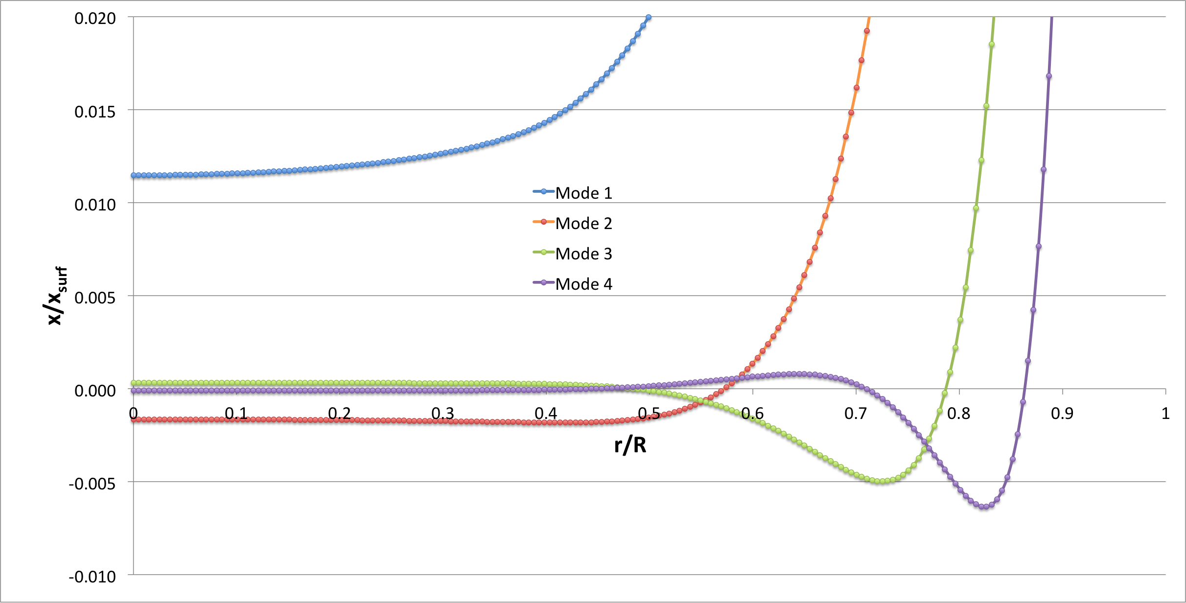
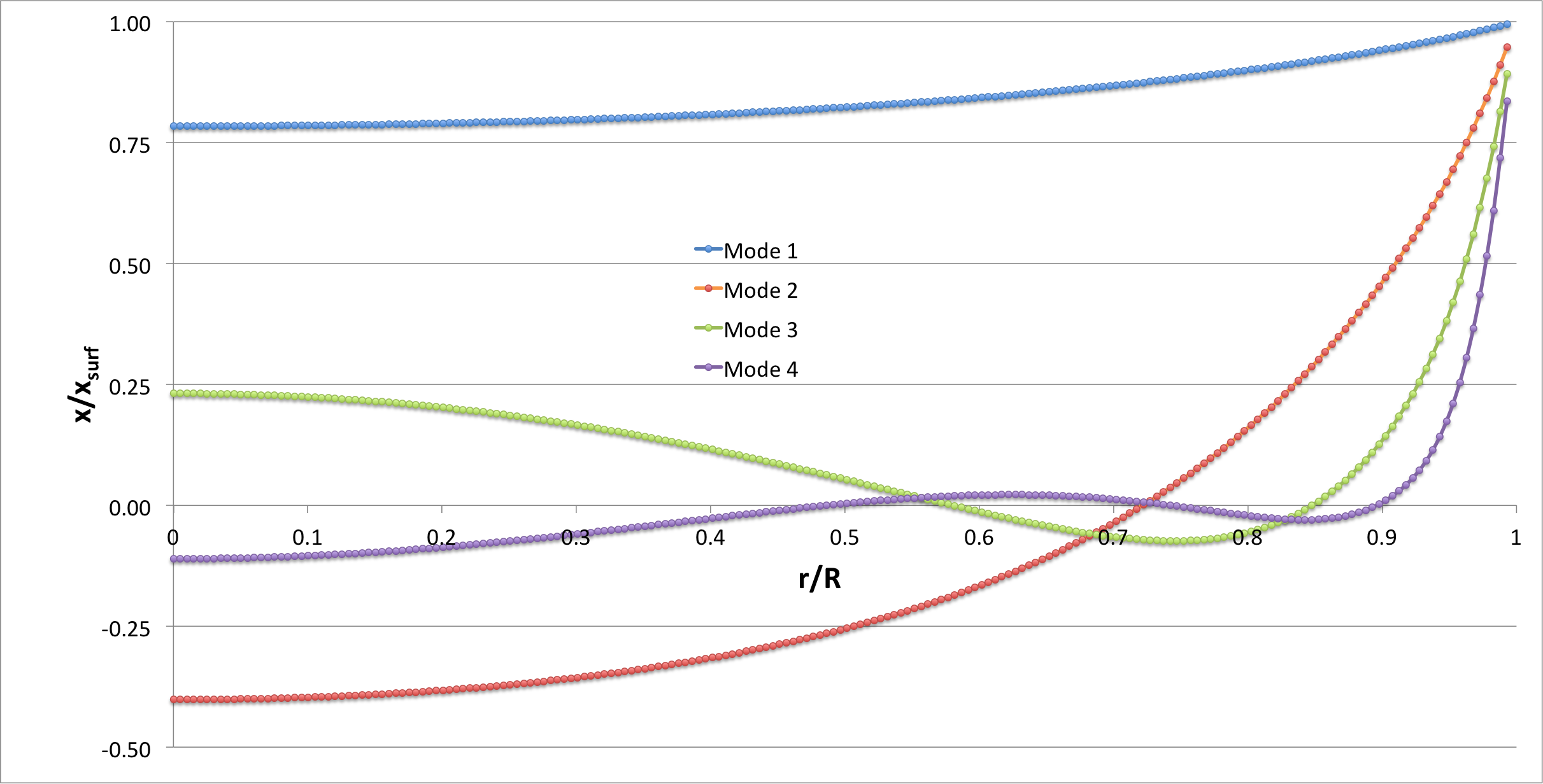
Keep in mind that, for all models, we expect that, at the surface, the logarithmic derivative of each proper eigenfunction will be,

<math>~\frac{d\ln x}{d\ln r^*}\biggr|_\mathrm{surf}</math>

<math>~=</math>

<math>~\frac{\Omega^2}{\gamma} - \alpha \, .</math>

Also, keep in mind that, for Model 10 <math>~(\xi_i = 2.5646)</math>:

<math>~\frac{r_i}{R}</math>

<math>~=</math>

<math>~0.39302482</math>

,

<math>~\frac{\rho_c}{\bar\rho}</math>

<math>~=</math>

<math>~34.3460405</math>

Our Determinations for Model 10
Mode	<math>~\sigma_c^2</math>	<math>~\Omega^2 \equiv \frac{\sigma_c^2}{2} \biggl( \frac{\rho_c}{\bar\rho}\biggr)</math>	<math>~x_\mathrm{surf}</math>	<math>~\frac{d\ln x}{d\ln r^*}\biggr|_\mathrm{surf}</math>		<math>~\frac{r}{R}\biggr|_1</math>	<math>~1 - \frac{M_r}{M_\mathrm{tot}}\biggr|_1</math>	<math>~\frac{r}{R}\biggr|_2</math>	<math>~1 - \frac{M_r}{M_\mathrm{tot}}\biggr|_2</math>	<math>~\frac{r}{R}\biggr|_3</math>	<math>~1 - \frac{M_r}{M_\mathrm{tot}}\biggr|_3</math>
				expected	measured
1 (Fundamental)	0.92813095170326	15.93881161	+85.17	8.963286966	8.963085	n/a	n/a	n/a	n/a	n/a	n/a
2	1.237156768978	21.24571822	- 610	12.14743093	12.147337	0.5724	3.05E-05	n/a	n/a	n/a	n/a
3	1.8656033984	32.0380449	+3225	18.62282676	18.6228	0.4845	1.35E-04	0.787	2.05E-07	n/a	n/a
4	2.65901504799	45.66331921	-9410	26.79799153	26.797977	0.4459	2.620E-04	0.7096	1.834E-06	0.8632	1.189E-08

For Model 17 <math>~(\xi_i = 3.0713)</math>:

<math>~\frac{r_i}{R}</math>

<math>~=</math>

<math>~0.93276717</math>

,

<math>~\frac{\rho_c}{\bar\rho}</math>

<math>~=</math>

<math>~3.79693903</math>

Our Determinations for Model 17
Mode	<math>~\sigma_c^2</math>	<math>~\Omega^2 \equiv \frac{\sigma_c^2}{2} \biggl( \frac{\rho_c}{\bar\rho}\biggr)</math>	<math>~x_\mathrm{surf}</math>	<math>~\frac{d\ln x}{d\ln r^*}\biggr|_\mathrm{surf}</math>		<math>~\frac{r}{R}\biggr|_1</math>	<math>~1 - \frac{M_r}{M_\mathrm{tot}}\biggr|_1</math>	<math>~\frac{r}{R}\biggr|_2</math>	<math>~1 - \frac{M_r}{M_\mathrm{tot}}\biggr|_2</math>	<math>~\frac{r}{R}\biggr|_3</math>	<math>~1 - \frac{M_r}{M_\mathrm{tot}}\biggr|_3</math>
				expected	measured
1 (Fundamental)	1.149837904	2.182932207	+1.275	0.7097593	0.7097550	n/a	n/a	n/a	n/a	n/a	n/a
2	7.34212930615	13.93880866	- 2.491	7.763285	7.763244	0.7215	0.24006	n/a	n/a	n/a	n/a
3	16.345072567	31.03062198	+4.33	18.01837	18.01826	0.5806	0.5027	0.848	0.0541	n/a	n/a
4	27.746934203	52.6767087	-9.1	31.0060	31.0058	0.4859	0.6737	0.7429	0.1974	0.8957	0.0171

Numerical Values for Some Selected <math>~(n_c, n_e) = (1, 5)</math> Bipolytropes [to be compared with Table 1 of Murphy & Fiedler (1985)]
MODEL	Source	<math>~\frac{r_i}{R}</math>	<math>~\Omega_0^2</math>	<math>~\Omega_1^2</math>	<math>~\frac{r}{R}\biggr|_1</math>	<math>~1-\frac{M_r}{M_\mathrm{tot}}\biggr|_1</math>
10	MF85	0.393	15.9298	21.2310	0.573	1.00E-03
	Here	0.39302	15.93881161	21.24571822	0.5724	3.05E-05
17	MF85	0.933	2.1827	13.9351	0.722	0.232
	Here	0.93277	2.182932207	13.93880866	0.7215	0.24006

Reconcile Approaches

Core:

Given that, <math>~\sqrt{2\pi}~r^* = \xi</math>, lets multiply the LAWE through by <math>~(2\pi)^{-1}</math>. This gives,

<math>~0</math>

<math>~=</math>

<math>~ \frac{d^2x}{d\xi^2} + \biggl\{ 4 -\biggl(\frac{\rho^*}{P^*}\biggr)\frac{ M_r^*}{(r^*)}\biggr\}\frac{1}{\xi} \cdot \frac{dx}{d\xi} + \frac{1}{2\pi}\biggl(\frac{\rho^*}{ P^* } \biggr)\biggl\{ \frac{2\pi \sigma_c^2}{3\gamma_\mathrm{g}} ~-~\frac{\alpha_\mathrm{g} M_r^*}{(r^*)^3}\biggr\} x \, . </math>

Specifically for the core, therefore, the finite-difference representation of the LAWE is,

<math>~\frac{x_+ -2x_j + x_-}{(\delta \xi)^2}</math>	<math>~=</math>	<math>~ -~ \frac{\mathcal{H}}{\xi} \biggl[ \frac{x_+ - x_-}{2\delta \xi} \biggr] ~-~ \biggl[ \frac{\mathcal{K}}{2\pi} \biggr]x_j </math>
<math>~\Rightarrow ~~~ x_+ -2x_j + x_-</math>	<math>~=</math>	<math>~ -~ \frac{\delta \xi}{2\xi} \biggl[ x_+ - x_- \biggr]\mathcal{H} ~-~ (\delta \xi)^2 \biggl[ \frac{\mathcal{K}}{2\pi} \biggr] x_j </math>
<math>~\Rightarrow ~~~ x_{j+1} \biggl[1 + \biggl( \frac{\delta \xi}{2\xi}\biggr) \mathcal{H} \biggr]</math>	<math>~=</math>	<math>~ \biggl[ 2 - (\delta \xi)^2\biggl( \frac{\mathcal{K}}{2\pi} \biggr) \biggr] x_j ~-~\biggl[ 1 - \biggl( \frac{\delta \xi}{2\xi} \biggr) \mathcal{H} \biggr]x_{j-1} \, . </math>

This also means that, as viewed from the perspective of the core, the slope at the interface is

<math>~\biggl[ \frac{dx}{d\xi}\biggr]_\mathrm{interface}</math>

<math>~=</math>

<math>~ \frac{1}{2\delta \xi} \biggl\{ \biggl[ 2 - (\delta \xi)^2 \biggl( \frac{\mathcal{K}}{2\pi} \biggr)\biggr] x_i ~-~2x_{i-1} \biggr\}\biggl[1 + \biggl( \frac{\delta \xi}{2\xi}\biggr) \mathcal{H} \biggr]^{-1} \, . </math>

Envelope:

Given that,

<math>~\biggl( \frac{\mu_e}{\mu_c} \biggr) \biggl(\frac{2\pi}{3}\biggr)^{1 / 2}~r^* = \eta \, ,</math>

let's multiply the LAWE through by <math>~(3/2\pi)( \mu_e/\mu_c)^{-2} </math>. This gives,

<math>~0</math>

<math>~=</math>

<math>~ \frac{d^2x}{d\eta^2} + \biggl\{ 4 -\biggl(\frac{\rho^*}{P^*}\biggr)\frac{ M_r^*}{(r^*)}\biggr\}\frac{1}{\eta} \cdot \frac{dx}{d\eta} + \frac{3}{2\pi} \biggl( \frac{\mu_e}{\mu_c} \biggr)^{-2} \biggl(\frac{\rho^*}{ P^* } \biggr)\biggl\{ \frac{2\pi \sigma_c^2}{3\gamma_\mathrm{g}} ~-~\frac{\alpha_\mathrm{g} M_r^*}{(r^*)^3}\biggr\} x \, . </math>

Specifically for the envelope, therefore, the finite-difference representation of the LAWE is,

<math>~\frac{x_+ -2x_j + x_-}{(\delta \eta)^2}</math>	<math>~=</math>	<math>~ -~ \frac{\mathcal{H}}{\eta} \biggl[ \frac{x_+ - x_-}{2\delta \eta} \biggr] ~-~ \biggl( \frac{\mu_e}{\mu_c} \biggr)^{-2}\biggl[ \frac{3\mathcal{K}}{2\pi} \biggr]x_j </math>
<math>~\Rightarrow ~~~ x_+ -2x_j + x_-</math>	<math>~=</math>	<math>~ -~ \frac{\delta \eta}{2\eta} \biggl[ x_+ - x_- \biggr]\mathcal{H} ~-~ (\delta \eta)^2 \biggl( \frac{\mu_e}{\mu_c} \biggr)^{-2}\biggl[ \frac{3\mathcal{K}}{2\pi} \biggr] x_j </math>
<math>~\Rightarrow ~~~ x_{j+1} \biggl[1 + \biggl( \frac{\delta \eta}{2\eta}\biggr) \mathcal{H} \biggr]</math>	<math>~=</math>	<math>~ \biggl[ 2 - (\delta \eta)^2 \biggl( \frac{\mu_e}{\mu_c} \biggr)^{-2} \biggl( \frac{3\mathcal{K}}{2\pi} \biggr) \biggr] x_j ~-~\biggl[ 1 - \biggl( \frac{\delta \eta}{2\eta} \biggr) \mathcal{H} \biggr]x_{j-1} \, . </math>

This also means that, once we know the slope at the interface (see immediately below), the amplitude at the first zone outside of the interface will be given by the expression,

<math>~x_{i+1} </math>

<math>~=</math>

<math>~ \biggl[ 1 - \tfrac{1}{2}(\delta \eta)^2 \biggl( \frac{\mu_e}{\mu_c} \biggr)^{-2} \biggl( \frac{3\mathcal{K}}{2\pi} \biggr)\biggr] x_i ~+~ \biggl[ 1 - \biggl( \frac{\delta \eta}{2\eta} \biggr) \mathcal{H} \biggr] \delta \eta \cdot \biggl[ \frac{dx}{d\eta} \biggr]_\mathrm{interface} \, . </math>

Interface

If we consider only cases where <math>~\gamma_e = \gamma_c</math>, then at the interface we expect,

<math>~\frac{d\ln x}{d\ln r^*}</math>	<math>~=</math>	<math>~\frac{d\ln x}{d\ln \xi} = \frac{d\ln x}{d\ln \eta}</math>
<math>~\Rightarrow ~~~ r^*\frac{dx}{d r^*}</math>	<math>~=</math>	<math>~\xi \frac{dx}{d \xi} = \eta \frac{d x}{d \eta}</math>
<math>~\Rightarrow ~~~ \frac{dx}{dr^*}</math>	<math>~=</math>	<math>~(2\pi)^{1 / 2}\frac{dx}{d\xi} = \biggl(\frac{\mu_e}{\mu_c}\biggr) \biggl(\frac{2\pi}{3}\biggr)^{1 / 2} \frac{dx}{d\eta} \, .</math>

Switching at the interface from <math>~\xi</math> to <math>~\eta</math> therefore means that,

<math>~ \biggl[ \frac{dx}{d\eta}\biggr]_\mathrm{interface}</math>

<math>~=</math>

<math>~\sqrt{3}\biggl(\frac{\mu_e}{\mu_c}\biggr)^{-1} \biggl[ \frac{dx}{d\xi}\biggr]_\mathrm{interface} \, .</math>

See Also

© 2014 - 2021 by Joel E. Tohline |   H_Book Home   |   YouTube   | Appendices: | Equations | Variables | References | Ramblings | Images | myphys.lsu | ADS | Recommended citation:   Tohline, Joel E. (2021), The Structure, Stability, & Dynamics of Self-Gravitating Fluids, a (MediaWiki-based) Vistrails.org publication, https://www.vistrails.org/index.php/User:Tohline/citation