User:Tohline/Appendix/Equation templates

Key Equations

Each of the equations displayed in the Tables, below, encapsulates a physical concept that is fundamental to our understanding of — and, hence our discussion of — the structure, stability, and dynamics of self-gravitating fluids. The pervasiveness of these physical concepts throughout astrophysics is reflected in the fact that the same equations — perhaps written in slightly different forms — appear in numerous published books and research papers. When attempting to understand the physical concept that is associated with any one of these mathematical relations, it can be helpful to read how and in what context different authors have introduced the expression in their own work. These Tables offer guides to some parallel discussions that have appeared in published texts over the past 5+ decades in connection with selected sets of key physical relations.

EXAMPLE: Suppose you want to gain a better understanding of the origin of the ideal gas equation of state, the definition of the gas constant <math>~\Re</math>, or how to determine the value of the mean molecular weight <math>~\bar{\mu}</math> of a gas. According to the Table entitled Equations of State, you will find a discussion of the ideal gas equation of state: near Eq. (1) in §II.1 of Chandrasekhar (1967); near Eq. (80.8) in §IX.80 of Landau & Lifshitz (1975); near Eq. (5.91) in Vol. I, §5.6 of Padmanabhan (2000); etc. A "note" (linked to a comment further down on this page) appears along with a table entry if the relevant equation in the cited reference contains notations or symbol names that differ significantly from the equation as displayed here.

Principal Governing Equations

Principal Governing Equations
To insert a given equation into any Wiki document, type ... {{ User:Tohline/Math/Template_Name }}		Parallel References § no. and (Eq. no.)
Template_Name	Resulting Equation	C67	LL75	H87	ST83	KW94	P00	BLRY07
EQ_Continuity01	Continuity Equation: <math>\frac{d\rho}{dt} + \rho \nabla \cdot \vec{v} = 0</math>		§I.1 (1.2) Note	§5.4 (5.37) Note	§6.1 (6.1.1) Note	§2.5 (2.22) Note	I: §8.5 (8.45)	§1.4 (1.53)
EQ_Euler01	Euler Equation: <math>\frac{d\vec{v}}{dt} = - \frac{1}{\rho} \nabla P - \nabla \Phi</math>		§I.2 (2.1) Note	§5.4 (5.38) Note	§6.1 (6.1.2)	§2.5 (2.20)	I: §8.5 (8.48)	§1.4 (1.55)
EQ_FirstLaw01	1st Law of Thermodynamics: <math>T \frac{ds}{dt} = \frac{d\epsilon}{dt} + P \frac{d}{dt} \biggl(\frac{1}{\rho}\biggr)</math>		§I.2 (2.5) Note	§4.2 (4.31) Note	§6.1 (6.1.8)	§4.1 (4.1) Note	I: §8.5 (8.53)
EQ_Poisson01	Poisson Equation: <math>\nabla^2 \Phi = 4\pi G \rho</math>		§I.3 (3.5) Note		§6.1 (6.1.4)	§1.3 (1.9)	I: §10.2 (10.1) Note	Chap. 7

Equations of State

Equations of State
To insert a given equation into any Wiki document, type ... {{ User:Tohline/Math/Template_Name }}		Parallel References § no. and (Eq. no.)
Template_Name	Resulting Equation	C67	LL75	H87	ST83	KW94	P00	BLRY07
EQ_EOSideal0A	Ideal Gas Equation of State: <math>~P_\mathrm{gas} = \frac{\Re}{\bar{\mu}} \rho T</math>	§II.1 (1) Note	§IX.80 (80.8) Note	§1.1 ("n")	§2.3 (2.3.32) or (3.2.12)	§13.0 (13.1) Note	I: §5.6 (5.91)	§5.4 (5.34)
EQ_ZTFG01	Degenerate Electron Pressure: <math>~P_\mathrm{deg} = A_\mathrm{F} F(\chi) </math> where:  <math>F(\chi) \equiv \chi(2\chi^2 - 3)(\chi^2 + 1)^{1/2} + 3\sinh^{-1}\chi</math> and:    <math>\chi \equiv (\rho/B_\mathrm{F})^{1/3}</math>   ———   NOTE:   ——— <math> F(\chi) = \frac{8}{5}\chi^5 - \frac{4}{7}\chi^7 + \cdots ~~~~~~(\mathrm{for}~~ \chi\ll 1) </math> <math> F(\chi) = 2\chi^4 - 2\chi^2 + \cdots ~~~~~~~(\mathrm{for}~~ \chi\gg 1) </math>	§X.1 (19) + (20)		§11.2 (11.41)	§2.3 (2.3.5) + (2.3.6)	§15.0 (15.13) + (15.14)	I: §5.9.2 (5.156) + (5.158)	§5.6.1 (5.86) + (5.87) + (5.88)
EQ_EOSradiation01	Radiation Pressure: <math>~P_\mathrm{rad} = \frac{1}{3} a_\mathrm{rad} T^4</math>			§12.1 (12.12) + (12.15)				§5.6.1 (5.85)
EQ_PressureTotal01	Normalized Total Pressure: <math>~p_\mathrm{total} = \biggl(\frac{\mu_e m_p}{\bar{\mu} m_u} \biggr) 8 \chi^3 \frac{T}{T_e} + F(\chi) + \frac{8\pi^4}{15} \biggl( \frac{T}{T_e} \biggr)^4</math>

Traditional Equations of (Spherical) Stellar Structure

Traditional Equations of (Spherical) Stellar Structure
To insert a given equation into any Wiki document, type ... {{ User:Tohline/Math/Template_Name }}		Parallel References § no. and (Eq. no.)
Template_Name	Resulting Equation	C67	LL75	H87	ST83	KW94	P00	BLRY07
EQ_SSmassConservation01	Mass Conservation: <math>~\frac{dM_r}{dr} = 4\pi r^2 \rho</math>	§IV.2 (6)			§3.2 (3.2.1)	§9.1 (9.1)	II: §2.2 (2.23)	§5.1 (5.2)
EQ_SShydrostaticBalance01	Hydrostatic Balance: <math>~\frac{dP}{dr} = - \frac{GM_r \rho}{r^2}</math>	§IV.2 (6)			§3.2 (3.2.2)	§9.1 (9.2) Note	II: §2.2 (2.22)	§5.1 (5.1)
EQ_SSLaneEmden01	Polytropic Lane-Emden Equation: <math>~\frac{1}{\xi^2} \frac{d}{d\xi}\biggl( \xi^2 \frac{d\Theta_H}{d\xi} \biggr) = - \Theta_H^n</math> Emden (1907) Ritter (1880)	§IV.2 (11) Note			§3.3 (3.3.6)	§19.2 (19.10)	I: §10.3 (10.4)
EQ_SSLaneEmden02	Isothermal Lane-Emden Equation: <math>~\frac{1}{\xi^2} \frac{d}{d\xi}\biggl( \xi^2 \frac{d\psi}{d\xi} \biggr) = e^{-\psi}</math>	§IV.22 (374)				§19.8 (19.35)	I: §10.3.3 (10.23)

 

Stability: Radial Pulsation

Stability: Radial Pulsation
To insert a given equation into any Wiki document, type ... {{ User:Tohline/Math/Template_Name }}		Parallel References § no. and (Eq. no.)
Template_Name	Resulting Equation	C67	ST83	KW94	HK99	P00
EQ_RadialPulsation01	LAWE:   Linear Adiabatic Wave (or Radial Pulsation) Equation <math>~ \frac{d^2x}{dr_0^2} + \biggl[\frac{4}{r_0} - \biggl(\frac{g_0 \rho_0}{P_0}\biggr) \biggr] \frac{dx}{dr_0} + \biggl(\frac{\rho_0}{\gamma_\mathrm{g} P_0} \biggr)\biggl[\omega^2 + (4 - 3\gamma_\mathrm{g})\frac{g_0}{r_0} \biggr] x = 0 </math> Eddington (1926)		§6.5 (6.5.6)	§38.1 (38.8)	§10.1.1 (10.16)	II: §3.7.1 (3.144)
EQ_RadialPulsation02	Polytropic LAWE: <math>~0 = \frac{d^2x}{d\xi^2} + \biggl[ 4 - (n+1) Q \biggr] \frac{1}{\xi} \cdot \frac{dx}{d\xi} + (n+1) \biggl[ \biggl( \frac{\sigma_c^2}{6\gamma_g } \biggr) \frac{\xi^2}{\theta} - \alpha Q\biggr] \frac{x}{\xi^2} </math> where:    <math>~Q(\xi) \equiv - \frac{d\ln\theta}{d\ln\xi} \, ,</math>    <math>~\sigma_c^2 \equiv \frac{3\omega^2}{2\pi G\rho_c} \, ,</math>     and,     <math>~\alpha \equiv \biggl(3 - \frac{4}{\gamma_\mathrm{g}}\biggr)</math>
EQ_RadialPulsation03	Isothermal LAWE: <math>~0 = \frac{d^2x}{d\xi^2} + \biggl[4 - \xi \biggl( \frac{d\psi}{d\xi} \biggr) \biggr] \frac{1}{\xi} \cdot \frac{dx}{d\xi} + \biggl[ \biggl( \frac{\sigma_c^2}{6\gamma_\mathrm{g}}\biggr)\xi^2 - \alpha \xi \biggl( \frac{d\psi}{d\xi} \biggr) \biggr] \frac{x}{\xi^2} </math> where:    <math>~\sigma_c^2 \equiv \frac{3\omega^2}{2\pi G\rho_c}</math>     and,     <math>~\alpha \equiv \biggl(3 - \frac{4}{\gamma_\mathrm{g}}\biggr)</math>

 

Special Function Relationships

Gamma Function

Gamma Function
To insert a given equation into any Wiki document, type ... {{ User:Tohline/Math/Template_Name }}		See also …
Template_Name	Resulting Equation
EQ_Gamma01	<math>~ \Gamma(z) ~\Gamma(1-z) </math> <math>~=</math> <math>~ \frac{\pi}{\sin(\pi z)} </math> <math>~\biggl|</math> for example, if <math>~z \rightarrow (m-n + \tfrac{1}{2})</math> <math>~\Rightarrow ~~~\Gamma(m-n+\tfrac{1}{2})~\Gamma(n-m+\tfrac{1}{2})</math> <math>~=</math> <math>~\pi \biggl\{\sin\biggl[ \frac{\pi}{2} + \pi(m-n) \biggr] \biggr\}^{-1}</math>   <math>~=</math> <math>~\pi (-1)^{m-n} </math> DLMF §5.5(ii) <math>~\biggl|</math> Valid for:    <math>~z \ne0, \pm 1, \pm 2, </math> … <math>~\biggl|</math>	A. Erdélyi (1953):  Volume I, §1.2, p. 3, eq. (6) Wikipedia

Toroidal Function Evaluations

Analytic Expressions & Plots

Toroidal Function Evaluations
To insert a given equation into any Wiki document, type ... {{ User:Tohline/Math/Template_Name }}		Graphical Representation (see:  generic caption)
Template_Name	Resulting Equation
EQ_PminusHalf01	<math>~P_{-\frac{1}{2}}(z)</math> <math>~=</math> <math>~ \frac{2}{\pi} \biggl[\frac{2}{z+1}\biggr]^{1 / 2} ~K\biggl( \sqrt{ \frac{z-1}{z+1}} \biggr) </math>       for example … <math>~P_{-\frac{1}{2}}(\cosh\eta)</math> <math>~=</math> <math>~ \biggl[ \frac{\pi}{2} \cdot \cosh \frac{\eta}{2} \biggr]^{-1} K\biggl( \tanh \frac{\eta}{2} \biggr) </math> Abramowitz & Stegun (1995), p. 337, eq. (8.13.1) Abramowitz & Stegun (1995), p. 337, eq. (8.13.2) NOTE: As we have explicitly demonstrated, an alternate, equivalent expression is <math>~P_{-\frac{1}{2}}(\cosh\eta)</math> <math>~=</math> <math>~\frac{\sqrt{2}}{\pi} (\sinh\eta)^{-1 / 2} k K(k)</math>       where:     <math>~k</math> <math>~\equiv</math> <math>~[2/(\coth\eta + 1)]^{1 / 2} \, .</math>
EQ_QminusHalf01	<math>~Q_{-\frac{1}{2}}(z)</math> <math>~=</math> <math>~ \sqrt{ \frac{2}{z+1} } ~K\biggl( \sqrt{ \frac{2}{z+1}} \biggr) </math>       for example … <math>~Q_{-\frac{1}{2}}(\cosh\eta)</math> <math>~=</math> <math>~ 2 e^{-\eta/2} K(e^{-\eta}) </math> Abramowitz & Stegun (1995), p. 337, eq. (8.13.3) Abramowitz & Stegun (1995), p. 337, eq. (8.13.4)
EQ_PplusHalf01	<math>~P_{+ \frac{1}{2}}(z)</math> <math>~=</math> <math>~ \frac{2}{\pi} \biggl[z + \sqrt{ z^2-1} \biggr]^{1 / 2} ~E\biggl( \sqrt{ \frac{2(z^2-1)^{1 / 2}}{z + (z^2-1)^{1 / 2}}} \biggr) </math>       for example … <math>~P_{+ \frac{1}{2}}(\cosh\eta)</math> <math>~=</math> <math>~ \frac{2}{\pi}~e^{\eta/2}~ E( \sqrt{1-e^{-2\eta}} ) </math> Abramowitz & Stegun (1995), p. 337, eq. (8.13.5) Abramowitz & Stegun (1995), p. 337, eq. (8.13.6)
EQ_QplusHalf01	<math>~Q_{+\frac{1}{2}}(z)</math> <math>~=</math> <math>~ z \sqrt{ \frac{2}{z+1} }~K\biggl( \sqrt{ \frac{2}{z+1} } \biggr) ~-~ [2(z+1)]^{1 / 2} E\biggl( \sqrt{ \frac{2}{z+1} } \biggr) </math> Abramowitz & Stegun (1995), p. 337, eq. (8.13.7)
EQ_Q1minusHalf01	<math>~Q^1_{-\frac{1}{2}}(z)</math> <math>~=</math> <math>~ - \biggl[\frac{1}{2(z-1)} \biggr]^{1 / 2} E(k) </math> where:   <math>~k = \sqrt{ \frac{2}{z+1}} \, .</math> (see our associated derivation)
EQ_Q2minusHalf01	<math>~Q^2_{-\frac{1}{2}}(z)</math> <math>~=</math> <math>~ \frac{ 4 z E(k) - (z-1) K(k) }{ [2^{3} (z+1) (z-1)^{2} ]^{1 / 2}} </math> where:   <math>~k \equiv \sqrt{ \frac{2}{z+1}} \, .</math> (see our associated derivation)

Caption for Plots

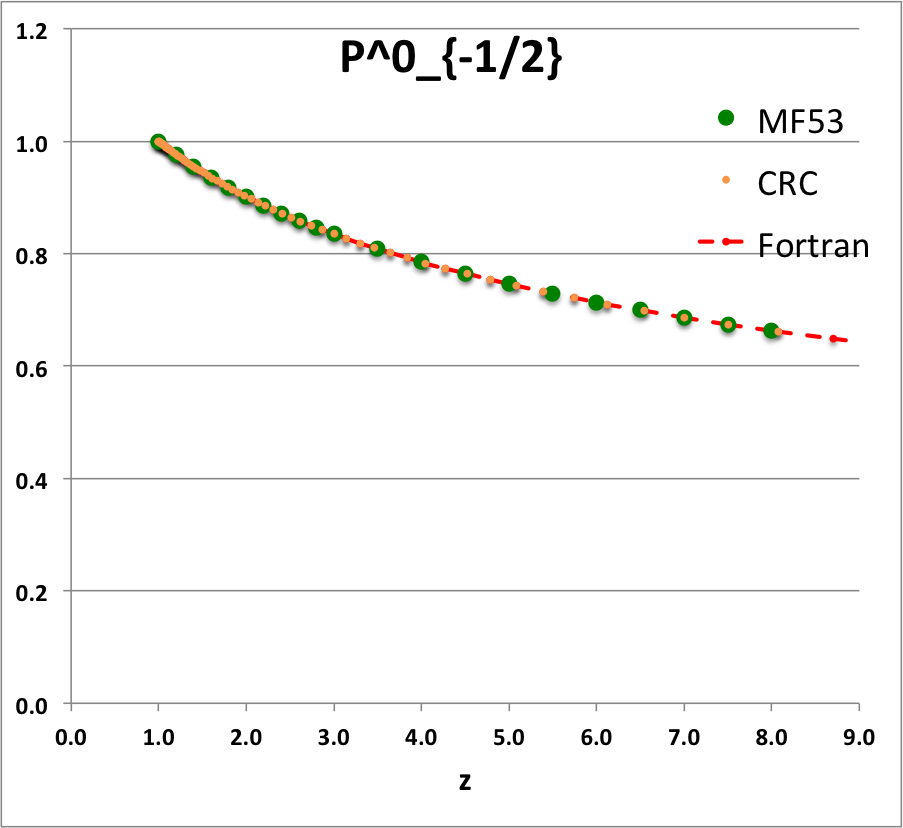
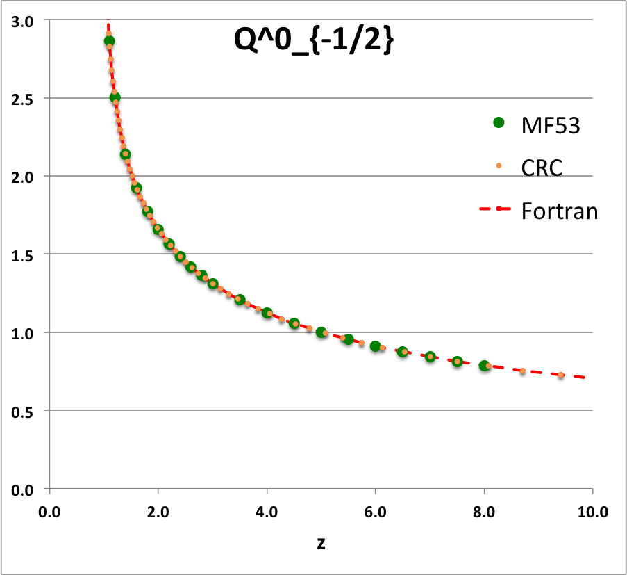
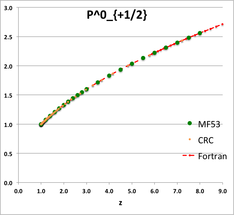
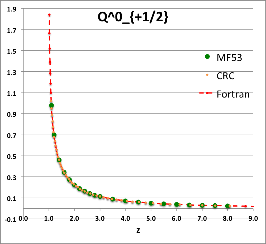
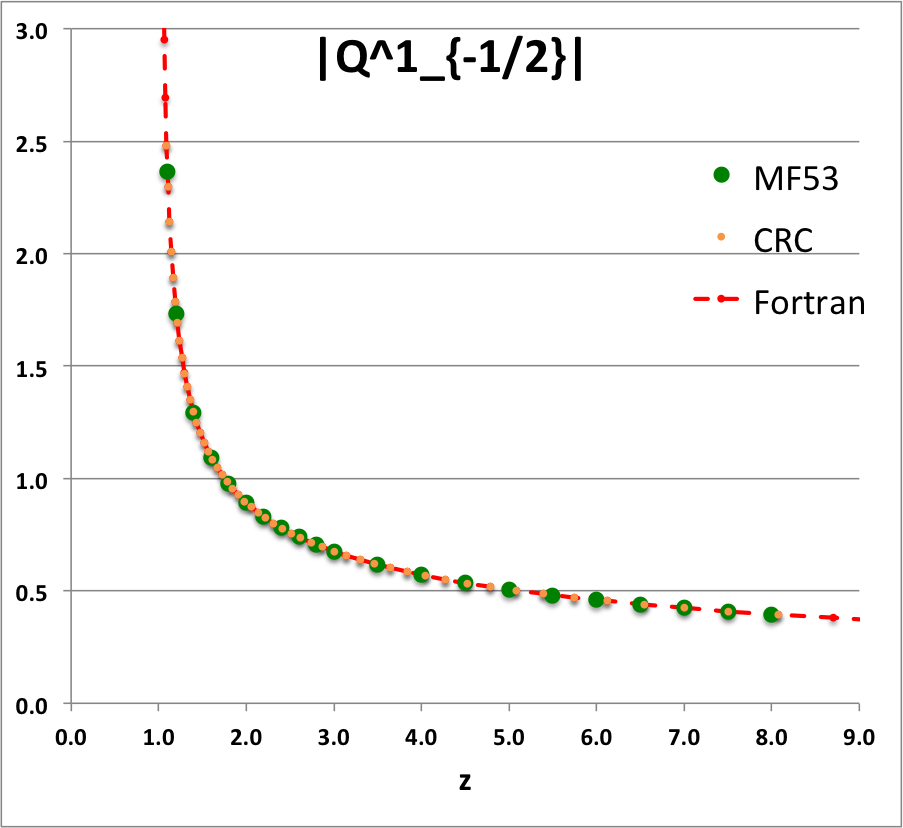
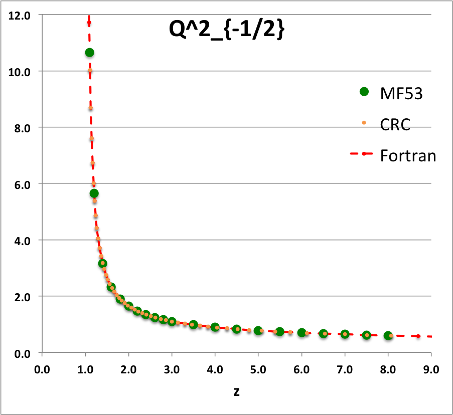
Caption for Plots:   Here we explain how we assembled the various plots — shown immediately above in the right-hand column of the "Toroidal Function Evaluations" table — that depict the behavior of various associated Legendre (toroidal) functions (see the related discussion) having varying half-integer degrees <math>~P^0_{-\frac{1}{2}}</math>, <math>~P^0_{+\frac{1}{2}}</math>, <math>~Q^0_{-\frac{1}{2}}</math>, <math>~Q^0_{+\frac{1}{2}}</math>, <math>~Q^0_{+\frac{3}{2}} \, ,</math> and (in association with a separate related discussion) having varying order <math>~Q^1_{-\frac{1}{2}}</math>, <math>~Q^2_{-\frac{1}{2}}</math>. For each choice of the integer indexes, <math>~n \ge 0</math> and <math>~m \ge 0</math>, the relevant plot shows how the function, <math>~X^n_{m-\frac{1}{2}}(z)</math>, varies with <math>~z</math>. In each plot … The solid green circular markers identify data that has been pulled directly from Table IX (p. 1923) of [MF53]; The solid orange circular markers identify function values that we have calculated using the relevant formulae as expressed herein in terms of the complete elliptic integrals, <math>~K(k)</math> and <math>~E(k)</math>, where the relevant values of the elliptic integrals have been pulled directly from tabulated values published in pp. 535 - 537 of the 1971 (19th) edition of the CRC's Standard Mathematical Tables, published by the Chemical Rubber Co., Cleveland, Ohio, U.S.A.. (See an accompanying sample of elliptic integral values extracted from this CRC handbook.) The dashed red curve was also derived using formulae expressed in terms of the complete elliptic integrals, but the values of the elliptic integrals have been calculated using (double-precision versions of) algorithms drawn from Numerical Recipes. NOTE: The tabulated values of the function, <math>~Q^1_{-\frac{1}{2}}</math>, that appear in Table IX (p. 1923) of [MF53] — see immediately below — are all positive, whereas, according to our derivation, they should all be negative. Therefore, for comparison purposes of this specific function — both here and in our accompanying discussion — we have plotted the absolute value of the function, <math>~|Q^1_{-\frac{1}{2}}(z)|</math>. ADDITIONAL NOTE:   In Example 4 on p. 340 of Abramowitz & Stegun (1995), we can pull one additional data point for comparison; specifically, they provide a high-precision evaluation of <math>~Q^0_{-\frac{1}{2}}(z = 2.6) = 1.419337751</math>. As can be seen in the table of function values immediately below, this is entirely consistent with the lower-precision value that we have extracted from [MF53], and exactly matches the double-precision value we have calculated based on the Numerical Recipes algorithm.

Example Recurrence Relations

The above Toroidal Function Evaluations table provides analytic expressions for the pair of foundation functions, <math>~P^0_{-\frac{1}{2}}(z)</math> and <math>~P^0_{+\frac{1}{2}}(z)</math>, and the associated pair of foundation functions, <math>~Q^0_{-\frac{1}{2}}(z)</math> and <math>~Q^0_{+\frac{1}{2}}(z)</math>. From either pair of foundation functions, expressions for all other zero-order, half-integer degree toroidal functions can be obtained using a relatively simple recurrence relation drawn from the "Key Equation,"

	<math>~(\nu - \mu + 1)P^\mu_{\nu + 1} (z)</math>	<math>~=</math>	<math>~ (2\nu + 1)z P_\nu^\mu(z) - (\nu + \mu)P^\mu_{\nu-1}(z) </math>
Abramowitz & Stegun (1995), p. 334, eq. (8.5.3)

NOTE: <math>~Q_\nu^\mu</math>, as well as <math>~P_\nu^\mu</math>, satisfies this same recurrence relation.

Specifically, letting <math>~\mu \rightarrow 0</math> and <math>~\nu \rightarrow (m - \tfrac{1}{2})</math>, for all <math>~m \ge 2</math>, we have,

<math>~P^0_{m-\frac{1}{2}}(z)</math>	<math>~=</math>	<math>~4 \biggl[ \frac{m-1}{2m-1} \biggr] z P^0_{m-\frac{3}{2}}(z) - \biggl[ \frac{2m-3}{2m-1}\biggr]P^0_{m-\frac{5}{2}}(z) \, ;</math>     and,
<math>~Q^0_{m-\frac{1}{2}}(z)</math>	<math>~=</math>	<math>~4 \biggl[ \frac{m-1}{2m-1} \biggr] z Q^0_{m-\frac{3}{2}}(z) - \biggl[ \frac{2m-3}{2m-1}\biggr]Q^0_{m-\frac{5}{2}}(z) \, .</math>

As examples, these two relations have been used to generate columns of numbers in the comparison table shown below for, respectively, the toroidal functions, <math>~P^0_{+\frac{3}{2}}(z)</math> and <math>~Q^0_{+\frac{3}{2}}(z)</math>. For order-1 and order-2 toroidal functions, the above table provides analytic expressions only for (the functions of the lowest half-integer degree) <math>~Q^1_{-\frac{1}{2}}(z)</math> and <math>~Q^2_{-\frac{1}{2}}(z)</math>. But, as we have detailed in an accompanying discussion, additional order-1 and order-2 expressions can be straightforwardly derived by drawing upon another key recurrence relation, namely,

	<math>~P_\nu^{\mu + 1}(z)</math>	<math>~=</math>	<math>~ (z^2-1)^{-\frac{1}{2}} \{ (\nu - \mu) z P^\mu_\nu(z) - (\nu + \mu)P^\mu_{\nu - 1}(z)\} </math>
Abramowitz & Stegun (1995), p. 333, eq. (8.5.1)

NOTE: <math>~Q_\nu^\mu</math>, as well as <math>~P_\nu^\mu</math>, satisfies this same recurrence relation.

Specifically, after adopting the association, <math>~\nu \rightarrow (n - \tfrac{1}{2})</math>, we have, when <math>~\mu = 0</math>,

<math>~Q_{n - \frac{1}{2}}^{1}(z)</math>

<math>~=</math>

<math>~ (n-\tfrac{1}{2}) (z^2-1)^{-\frac{1}{2}} [z Q_{n - \frac{1}{2}}(z) - Q_{n - \frac{3}{2}}(z)] </math>

…

for <math>~n \ge 1 \, ,</math>

and, when <math>~\mu = 1</math>,

<math>~Q_{n - \frac{1}{2}}^{2}(z)</math>

<math>~=</math>

<math>~ (z^2-1)^{-\frac{1}{2}} \{ (n-\tfrac{3}{2}) z Q^1_{n - \frac{1}{2}}(z) - (n+\tfrac{1}{2})Q^1_{n - \frac{3}{2}}(z)\} </math>

…

for <math>~n \ge 1 \, .</math>

As an example, the first of these two relations has been used to generate a column of numbers in the comparison table shown below for the toroidal function, <math>~Q^1_{+\frac{1}{2}}(z)</math>.

Comparison with Table IX from MF53

To facilitate copying & pasting for immediate use by other researchers, here we present in a tab-delimited, plain-text format the evaluation of nine separate toroidal functions: (Top half of table) <math>~P^0_{-\frac{1}{2}}</math>, <math>~P^0_{+\frac{1}{2}}</math> and <math>~P^0_{+\frac{3}{2}}</math>; (Bottom half of table) <math>~Q^0_{-\frac{1}{2}}</math>, <math>~Q^1_{-\frac{1}{2}}</math>, <math>~Q^2_{-\frac{1}{2}}</math>, <math>~Q^0_{+\frac{1}{2}}</math>, <math>~Q^1_{+\frac{1}{2}}</math> and <math>~Q^0_{+\frac{3}{2}}</math>. Each function has been evaluated for approximately 23 different argument values in the range, <math>~1.0 \le z \le 9.0</math>, and, for each function, two columns of function values have been presented: (Left column) Low-precision evaluation extracted directly from Table IX (p. 1923) of [MF53]; (Right column) Our double-precision evaluation based on a set of Numerical Recipes algorithms. One exception: The value listed under the "MF53" column for the evaluation of <math>~Q^0_{-\frac{1}{2}}(z=2.6)</math> is the high-precision value published on p. 340 of Abramowitz & Stegun (1995); notice that our high-precision evaluation matches all ten digits of their published value.

Top half of Table IX (p. 1923) of [MF53]

z P0m1Half(z) P0p1Half(z) P0p3Half(z) MF53 Our Calc. MF53 Our Calc. MF53 Our Calc. 1.0 1.0000 1.0000 1.0000 1.2 0.9763 9.763155118E-01 1.0728 1.072784040E+00 1.3910 1.391015961E+00 1.4 0.9549 9.549467781E-01 1.1416 1.141585331E+00 1.8126 1.812643692E+00 1.6 0.9355 9.355074856E-01 1.2070 1.206963827E+00 2.2630 2.263020336E+00 1.8 0.9177 9.176991005E-01 1.2694 1.269362428E+00 2.7406 2.740570128E+00 2.0 0.9013 9.012862994E-01 1.3291 1.329138155E+00 3.2439 3.243939648E+00 2.2 0.8861 8.860804115E-01 1.3866 1.386583505E+00 3.7719 3.771951476E+00 2.4 0.8719 8.719279330E-01 1.4419 1.441941436E+00 4.3236 4.323569952E+00 2.6 0.8587 8.587023595E-01 1.4954 1.495416274E+00 4.8979 4.897875630E+00 2.8 0.8463 8.462982520E-01 1.5472 1.547181667E+00 5.4941 5.494045473E+00 3.0 0.8346 8.346268417E-01 1.5974 1.597386605E+00 6.1113 6.111337473E+00 3.5 0.8082 8.081851582E-01 1.7169 1.716877977E+00 7.7427 7.742702172E+00 4.0 0.7850 7.849616703E-01 1.8290 1.828992729E+00 9.4930 9.492973996E+00 4.5 0.7643 7.643076802E-01 1.9349 1.934919997E+00 11.3555 1.135475076E+01 5.0 0.7457 7.457491873E-01 2.0356 2.035563839E+00 13.3220 1.332184253E+01 5.5 0.7289 7.289297782E-01 2.1316 2.131629923E+00 15.3890 1.538897617E+01 6.0 0.7136 7.135750093E-01 2.2237 2.223681177E+00 17.5520 1.755159108E+01 6.5 0.6995 6.994692725E-01 2.3122 2.312174942E+00 19.8060 1.980569307E+01 7.0 0.6864 6.864402503E-01 2.3975 2.397488600E+00 22.1480 2.214774685E+01 7.5 0.6743 6.743481630E-01 2.4799 2.479937758E+00 24.5750 2.457459486E+01 8.0 0.6631 6.630781433E-01 2.5598 2.559789460E+00 27.0830 2.708339486E+01 8.5 6.525347093E-01 2.637271986E+00 2.967157094E+01 9.0 6.426376817E-01 2.712582261E+00 3.233677457E+01

Bottom half of Table IX (p. 1923) of [MF53]

z Q0m1Half(z) Q1m1Half(z) Q2m1Half(z) Q0p1Half(z) Q1p1Half(z) Q0p3Half(z) MF53 Our Cal. MF53 Our Calc. MF53 Our Calc. M53 Our Calc. MF53 Our Calc. MF53 Our Calc. 1.1 2.8612 2.861192872E+00 2.3661 -2.366084077E+00 10.6440 1.064378304E+01 0.9788 9.787602829E-01 1.9471 -1.947110839E+00 0.4818 4.817841242E-01 1.2 2.5010 2.500956508E+00 1.7349 -1.734890983E+00 5.6518 5.651832631E+00 0.6996 6.995548314E-01 1.2524 -1.252395745E+00 0.2856 2.856355610E-01 1.4 2.1366 2.136571733E+00 1.2918 -1.291802851E+00 3.1575 3.157491205E+00 0.4598 4.597941602E-01 0.7618 -7.618218821E-01 0.14609 1.460918547E-01 1.6 1.9229 1.922920866E+00 1.0943 -1.094337965E+00 2.3230 2.323018870E+00 0.3430 3.430180260E-01 0.5501 -5.500770475E-01 0.09080 9.079816684E-02 1.8 1.7723 1.772268479E+00 0.9748 -9.748497733E-01 1.9018 1.901788930E+00 0.2720 2.720401772E-01 0.4285 -4.284853031E-01 0.06214 6.214026586E-02 2.0 1.6566 1.656638170E+00 0.8918 -8.917931374E-01 1.6454 1.645348489E+00 0.2240 2.240142929E-01 0.3489 -3.488955345E-01 0.04516 4.515872426E-02 2.2 1.5634 1.563378886E+00 0.8293 -8.292825549E-01 1.4712 1.471197798E+00 0.18932 1.893229696E-01 0.29263 -2.926294028E-01 0.03422 3.422108228E-02 2.4 1.4856 1.485653983E+00 0.7798 -7.797558474E-01 1.3441 1.344108936E+00 0.16312 1.631167365E-01 0.25076 -2.507568731E-01 0.02676 2.675556229E-02 2.6 1.419337751 1.419337751E+00 0.7391 -7.390875295E-01 1.2465 1.246521876E+00 0.14266 1.426580119E-01 0.21842 -2.184222751E-01 0.02143 2.143519083E-02 2.8 1.3617 1.361744950E+00 0.7048 -7.048053314E-01 1.1687 1.168702464E+00 0.12628 1.262756033E-01 0.19274 -1.927423405E-01 0.01751 1.751393553E-02 3.0 1.3110 1.311028777E+00 0.6753 -6.753219405E-01 1.1048 1.104816977E+00 0.11289 1.128885424E-01 0.17189 -1.718911443E-01 0.01454 1.454457729E-02 3.5 1.2064 1.206444997E+00 0.6163 -6.163068170E-01 0.9846 9.846190928E-01 0.08824 8.824567577E-02 0.13380 -1.338040913E-01 0.00966 9.664821286E-03 4.0 1.1242 1.124201960E+00 0.5713 -5.712994484E-01 0.8990 8.990205764E-01 0.07154 7.154134054E-02 0.10819 -1.081900595E-01 0.00682 6.819829619E-03 4.5 1.0572 1.057164923E+00 0.5353 -5.353494651E-01 0.8339 8.338659751E-01 0.05957 5.956966068E-02 0.08993 -8.992645608E-02 0.00503 5.029656514E-03 5.0 1.0011 1.001077380E+00 0.5057 -5.056928088E-01 0.7820 7.819717783E-01 0.05063 5.062950976E-02 0.07634 -7.633526879E-02 0.00384 3.837604899E-03 5.5 0.9532 9.532056775E-01 0.4806 -4.806378723E-01 0.7393 7.392682950E-01 0.04374 4.373774515E-02 0.06588 -6.588433822E-02 0.00301 3.008238619E-03 6.0 0.9117 9.116962715E-01 0.4591 -4.590784065E-01 0.7033 7.032568965E-01 0.03829 3.828867029E-02 0.05764 -5.763649873E-02 0.00241 2.410605139E-03 6.5 0.87524 8.752387206E-01 0.44025 -4.402537373E-01 0.67231 6.723067009E-01 0.03389 3.389003482E-02 0.05099 -5.098806037E-02 0.00197 1.967394932E-03 7.0 0.84288 8.428751774E-01 0.42362 -4.236198508E-01 0.64530 6.453008278E-01 0.03028 3.027740449E-02 0.04553 -4.553369214E-02 0.00163 1.630716095E-03 7.5 0.81389 8.138862008E-01 0.40877 -4.087751846E-01 0.62144 6.214442864E-01 0.02727 2.726650960E-02 0.04099 -4.099183107E-02 0.00137 1.369695722E-03 8.0 0.78772 7.877190099E-01 0.39542 -3.954155185E-01 0.60015 6.001530105E-01 0.02473 2.472532098E-02 0.03716 -3.716124286E-02 0.00116 1.163753807E-03 8.5 7.639406230E-01 -3.833053056E-01 5.809864341E-01 2.255696890E-02 -3.389458114E-02 9.987731857E-04 9.0 7.422062367E-01 -3.722587645E-01 5.636047532E-01 2.068890884E-02 -3.108168349E-02 8.648271474E-04

Relationships Between Various Associated Legendre Functions

Relationships Between Various Associated Legendre Functions
To insert a given equation into any Wiki document, type ... {{ User:Tohline/Math/Template_Name }}		See also …
Template_Name	Resulting Equation
EQ_Toroidal01	<math>~ Q_\nu[t t^' - (t^2-1)^{1 / 2} (t^{'2} - 1)^{1 / 2} \cos\psi] </math> <math>~=</math> <math>~ Q_\nu(t) P_\nu(t^') + 2\sum_{n=1}^\infty (-1)^n Q^n_\nu(t) P^{-n}_\nu(t^') \cos(n\psi) </math> A. Erdélyi (1953):  Volume I, §3.11, p. 169, eq. (4) Valid for:     <math>~t, t^'</math>  real         <math>~1 < t^' < t</math>         <math>~\nu \ne -1, -2, -3, </math> …         <math>~\psi</math>   real	T. G. Cowling (1940):   p. 223 (note sign discrepancy in argument of <math>~Q_\nu</math>) DLMF §14.18.5
EQ_Toroidal02	<math>~Q_{n-1 / 2}^m (\lambda)</math> <math>~=</math> <math>~(-1)^n \frac{\pi^{3/2}}{\sqrt{2}~ \Gamma(n-m+1 / 2)} (x^2-1)^{1 / 4} P_{m-1 / 2}^n(x) \, , </math> Gil, Segura, & Temme (2000):  eq. (8) where:     <math>~\lambda \equiv x/\sqrt{x^2-1}</math>	Cohl et al. (2000), eq. (34) DLMF §14.19.v together with DLMF §14.3.10
EQ_Toroidal03	<math>~Q_\nu^\mu(z)</math> <math>~=</math> <math>~ e^{i \mu \pi} ~ (2\pi)^{-\frac{1}{2}} (z^2-1)^{\mu/2} ~\Gamma(\mu + \tfrac{1}{2})~\biggl\{ \int_0^\pi (z - \cos t)^{-\mu - \frac{1}{2}} \cos[(\nu + \tfrac{1}{2})t] ~dt -\cos(\nu\pi) \int_0^\infty (z + \cosh t)^{-\mu - \frac{1}{2}} e^{-(\nu + \frac{1}{2})t} ~dt \biggr\} </math> A. Erdélyi (1953):  Volume I, §3.7, p. 156, eq. (10) Valid for:     <math>~\mathrm{Re} ~\nu > -\tfrac{1}{2}</math>      and     <math>~\mathrm{Re} (\nu + \mu + 1) > 0 \, .</math>
EQ_Toroidal04	<math>~(\nu - \mu + 1)P^\mu_{\nu + 1} (z)</math> <math>~=</math> <math>~ (2\nu + 1)z P_\nu^\mu(z) - (\nu + \mu)P^\mu_{\nu-1}(z) </math> Abramowitz & Stegun (1995), p. 334, eq. (8.5.3) NOTE: <math>~Q_\nu^\mu</math>, as well as <math>~P_\nu^\mu</math>, satisfies this same recurrence relation.	Cohl & Tohline (1999), §2.2.2, eq. (25) Guatschi (1965), p. 490, procedure toroidal
EQ_Toroidal05	<math>~ \int_a^b\biggl[(\nu - \sigma)(\nu + \sigma + 1) + (\rho^2 - \mu^2)(1 - z^2)^{-1} \biggr] w_\nu^\mu ~w_\sigma^\rho ~dz </math> <math>~=</math> <math>~ \biggl[ z(\nu-\sigma) w_\nu^\mu ~w_\sigma^\rho + (\sigma+\rho) w_\nu^\mu ~ w_{\sigma-1}^\rho - (\nu + \mu) w_{\nu - 1}^\mu ~w_\sigma^\rho \biggr]_a^b </math> A. Erdélyi (1953):  Volume I, §3.12, p. 169, eq. (1) where, <math>~w_\nu^\mu(z)</math> and <math>~w_\sigma^\rho(z)</math> denote any solutions of Legendre's differential equation
EQ_Toroidal06	<math>~(\xi - z)\sum_{m=0}^n (2m+1)P_m(z) Q_m(\xi)</math> <math>~=</math> <math>~ 1 - (\ell+1)[P_{\ell+1}(z) Q_\ell(\xi) - P_\ell(z)Q_{\ell+1}(\xi)] </math> Abramowitz & Stegun (1995), p. 335, eq. (8.9.2)	Erdélyi (1953):  Volume I, §3.8, p. 162, eq. (21)
EQ_Toroidal07	<math>~P_\nu^{\mu + 1}(z)</math> <math>~=</math> <math>~ (z^2-1)^{-\frac{1}{2}} \{ (\nu - \mu) z P^\mu_\nu(z) - (\nu + \mu)P^\mu_{\nu - 1}(z)\} </math> Abramowitz & Stegun (1995), p. 333, eq. (8.5.1) NOTE: <math>~Q_\nu^\mu</math>, as well as <math>~P_\nu^\mu</math>, satisfies this same recurrence relation.
EQ_Toroidal08	<math>~ Q_{-\frac{1}{2}}^\mu(z) + 2\sum_{n=1}^\infty Q^\mu_{n-\frac{1}{2}}(z) \cos(n\nu) </math> <math>~=</math> <math>~ e^{i\mu\pi}~\biggl(\frac{\pi}{2} \biggr)^{1 / 2} \Gamma(\mu + \tfrac{1}{2})\biggl[ \frac{(z^2-1)^{\mu/2}}{(z - \cos\nu)^{\mu + \frac{1}{2}}} \biggr] </math> A. Erdélyi (1953):  Volume I, §3.10, p. 166, eq. (3) Valid for:     <math>~\mathrm{Re}~\mu > - \tfrac{1}{2}</math>

 

Key Parallel References (printed texts spanning 5+ decades)

• [C67] Chandrasekhar, S. 1967 (originally, 1939), An Introduction to the Study of Stellar Structure (New York: Dover)
  • EQ_EOSideal0A — In C67, the ideal gas equation of state is initially written in terms of the specific volume <math>~V</math>, instead of the mass density <math>~\rho</math>; also, it is initially assumed that <math>~\bar{\mu}</math> = 1. Both <math>~\rho</math> and <math>~\bar{\mu}</math> are introduced in §III.1, Eq.(5).
  • EQ_SSLaneEmden01 — At the end of his Chapter IV, C67 writes an extensive history of the earliest work on stellar structure pointing especially the origins of the so-called Lane-Emden equation. He points out, for example, that Ritter (1880) actually published this governing differential equation prior to Emden.

• [LL75] Laundau, L. D. & Lifshitz, E. M. 1975 (originally, 1959), Fluid Mechanics (New York: Pergamon Press)
  • EQ_Continuity01 — LL75 present the Eulerian, rather than the Lagrangian form of the Continuity equation.
  • EQ_Euler01 — In the Euler equation, LL75 do not initially include a source term to account for a gradient in the Newtonian gravitational potential, <math>~\Phi</math>; a term representing acceleration due to gravity, <math>\vec{g} = -\nabla\Phi</math>, is introduced in Eq.(2.4), but in LL75 this is intended primarily to describe gravity at the surface of the Earth.
  • EQ_FirstLaw01 — LL75's Eq.(2.5) must be combined with their discussion of what they refer to as the familiar thermodynamic relation (between LL75 Eqs. 2.8 and 2.9) in order to appreciate the similarity with our expression.
  • EQ_Poisson01 — In LL75, the symbol <math>\Delta</math>, rather than <math>\nabla^2</math>, is used to represent the Laplacian spatial operator.
  • EQ_EOSideal0A — In LL75, the ideal gas equation of state is written in terms of the specific volume <math>~V</math>, as well as in terms of the mass density <math>~\rho</math>.

• [ST83] Shapiro, S. L. & Teukolsky, S. A. 1983, Black Holes, White Dwarfs, and Neutron Stars: The Physics of Compact Objects (New York: John Wiley & Sons); republished in 2004 by WILEY-VCH Verlag GmbH & Co. KGaA
  • EQ_Continuity01 — ST83 present the Eulerian, rather than the Lagrangian form of the Continuity equation.

• [H87] Huang, K. 1987 (originally 1963), Statistical Mechanics (New York: John Wiley & Sons)
  • EQ_Continuity01 — H87 presents the Eulerian, rather than the Lagrangian form of the Continuity equation, and the variable <math>\vec{u}</math> is used instead of <math>~\vec{v}</math> to represent the velocity.
  • EQ_Euler01 — H87 presents the Eulerian, rather than the Lagrangian form of the Euler equation, and the variable <math>\vec{u}</math> is used instead of <math>~\vec{v}</math> to represent the velocity. Furthermore, to match the source term in our version of the Euler equation, we must set H87's applied acceleration, <math>\vec{F}/m = -\nabla</math><math>~\Phi</math>.
  • EQ_FirstLaw01 — H87 begins a discussion of the 1^st Law of Thermodynamics in the first section of the first chapter, but it does not appear in the form we present (relevant for a "dilute gas") until Eq.(4.31).

• [BT87] Binney, J. & Tremaine, S. 1987, Galactic Dynamics (Princeton, NJ: Princeton University Press)

• [KW94] Kippenhahn, R. & Weigert, A. 1994, Stellar Structure and Evolution (New York: Springer-Verlag)
  • EQ_Continuity01 — KW94 present the Eulerian, rather than the Lagrangian form of the Continuity equation.
  • EQ_FirstLaw01 — In KW94, the symbol <math>u</math> instead of <math>~\epsilon</math> is used to represent the specific internal energy.
  • EQ_EOSideal0A — In KW94, the ideal gas equation of state is actually first introduced in §2.2, Eq.(27), but it is seriously discussed in Chapter 13. KW94 provide a particularly nice explanation of how to calculate the model parameter, <math>~\bar{\mu}</math>.
  • EQ_SShydrostaticBalance01 — In KW94, the hydrostatic balance equation is expressed in terms of <math>dP/dM_r</math> instead of <math>dP/dr</math>; and the second term on the right-hand-side allows for a net radial acceleration.

• [HK99] Hansen, C. J. & Kawaler, S. D. 1999, Stellar Interiors: Physical Principles, Structure, and Evolution (New York: Springer)

• [P00] Padmanabhan, T. 2000, Theoretical Astrophysics. Volume I: Astrophysical Processes (Cambridge: Cambridge University Press); and Padmanabhan, T. 2001, Theoretical Astrophysics. Volume II: Stars and Stellar Systems (Cambridge: Cambridge University Press)
  • EQ_Poisson01 — See also Vol.I: §10.4, Eq.(10.58).

• [BLRY07] Bodenheimer, P., Laughlin, G. P., Różyczka, M. & Yorke, H. W. 2007, Numerical Methods in Astrophysics An Introduction (New York: Taylor & Francis)

Other Equations with Assigned Templates

To insert a given equation into any Wiki document, type ... {{ User:Tohline/Math/Template_Name }}
Template_Name	Resulting Equation	Description
EQ_Continuity02	<math>~\frac{\partial\rho}{\partial t} + \nabla \cdot (\rho \vec{v}) = 0</math>	Eulerian (and Conservative) form of the continuity equation.
EQ_Euler02	<math>~\frac{\partial\vec{v}}{\partial t} + (\vec{v}\cdot \nabla) \vec{v}= - \frac{1}{\rho} \nabla P - \nabla \Phi</math>	Eulerian form of the Euler equation.
EQ_Euler03	<math>~\frac{\partial(\rho\vec{v})}{\partial t} + \nabla\cdot [(\rho\vec{v})\vec{v}]= - \nabla P - \rho \nabla \Phi</math>	Conservative form of the Euler equation.
EQ_Euler04	<math>~\frac{\partial\vec{v}}{\partial t} + \vec\zeta \times \vec{v}= - \frac{1}{\rho} \nabla P - \nabla \biggl[\Phi + \frac{1}{2}v^2 \biggr] </math>	Euler equation in terms of vorticity.
EQ_FirstLaw02	<math>~\frac{d\epsilon}{dt} + P \frac{d}{dt} \biggl(\frac{1}{\rho}\biggr) = 0</math>	Adiabatic form of the 1st Law of Thermodynamics.
EQ_Polytrope01	<math>~P = K_\mathrm{n} \rho^{1+1/n}</math>	Polytropic equation of state.
EQ_Polytrope02	<math>~H = (n+1)K_\mathrm{n} \rho^{1/n}</math>	Enthalpy in a polytrope.
EQ_Polytrope03	<math>~\rho = \biggl[ \frac{H}{(n+1)K_\mathrm{n}} \biggr]^n </math>	Density in terms of enthalpy for polytrope.
EQ_EOSideal00	<math>~P = n_g k T</math>	Alternate form of the ideal gas equation of state.
EQ_EOSideal02	<math>~P = (\gamma_\mathrm{g} - 1)\epsilon \rho </math>	Alternate form of the ideal gas equation of state.
EQ_TRApproximation	<math>~\Phi_\mathrm{TR}(\varpi,z)</math> <math>~=</math> <math>~-\biggl[ \frac{2GM}{\pi } \biggr]\frac{K(k)}{\sqrt{(\varpi+a)^2 + z^2}}</math> <math>\mathrm{where:}~~~k \equiv \{4\varpi a/[ (\varpi+a)^2 + z^2]\}^{1 / 2}</math>	Gravitational potential exterior to an axisymmetric torus, in the Thin Ring (TR) Approximation.
EQ_CT99Axisymmetric	<math>~\Phi(\varpi,z)\biggr|_\mathrm{axisym}</math> <math>~=</math> <math>~ - \frac{G}{\pi} \iint\limits_\mathrm{config} \biggl[ \frac{\mu}{(\varpi~ \varpi^')^{1 / 2}} \biggr] K(\mu) \rho(\varpi^', z^') 2\pi \varpi^'~ d\varpi^' dz^' </math> <math>\mathrm{where:}~~~\mu \equiv \{4\varpi \varpi^' /[ (\varpi+\varpi^')^2 + (z-z^')^2]\}^{1 / 2}</math>	Gravitational potential of any axisymmetric mass distribution.

 

 

© 2014 - 2021 by Joel E. Tohline |   H_Book Home   |   YouTube   | Appendices: | Equations | Variables | References | Ramblings | Images | myphys.lsu | ADS | Recommended citation:   Tohline, Joel E. (2021), The Structure, Stability, & Dynamics of Self-Gravitating Fluids, a (MediaWiki-based) Vistrails.org publication, https://www.vistrails.org/index.php/User:Tohline/citation