Simple Cube Tutorial

Getting Started

As in §4.1 (p. 38) of the VTK User's Guide, authored and published by Kitware, Inc., we will start off by rendering a simple cylinder.

1. Inside VisTrails, open, then execute "Cylinder.vt" without making any changes to the default pipeline or to any module parameters:

Follow this directory path: VisTrails/examples/vtk_examples/Rendering/Cylinder.vt
Upon execution, the image that pops up in the VisTrails spreadsheet window will be totally orange (actually, the color is "tomato") and will not look like a cylinder. This is because the default position of the camera places you inside the tomato-colored cylinder.
You can view the cylinder by placing your mouse cursor inside the relevant spreadsheet window and using the appropriate mouse control to "zoom out". Then other mouse actions will let you spin the cylinder and/or move it side to side.

Cylinder01

2. Modify the initial camera position:

Click on the "vtkCamera" module of the Cylinder.vt Pipeline; the "Methods" segment of the VisTrails Builder Window will list all of the methods that can be activated within the vtkCamera module.
Note that, in the bottom half of this "Methods" window segment, the "Zoom" method has already been activated with a value of 1.5.
Scroll through the list of methods to find the "SetPosition" method; highlight that method and drag it into the bottom half (Set Methods) segment of the Methods window; three empty "Float" text windows will appear, allowing you to enter floating-point numbers to specify, respectively, the <math>x</math>, <math>y</math>, and <math>z</math> coordinates of the desired camera position.
Type 5.0, 5.0, and 5.0 into the three "Float" text windows, then execute the Cylinder.vt Pipeline again; this should produce the tipped, 8-sided, tomato-colored cylinder (on a dark blue background) shown here as Fig. Cylinder01.

3. Play with the prescribed values of other method parameters:

Click on the "vtkCylinderSource" module and note that the "SetResolution" method has a default integer value of 8; this is why the generated cylinder is not round but, instead, is 8-sided.
- Change the "SetResolution" value from, say, 8 to 20, then re-execute the Cylinder.vt pipeline.
- Drag the "SetRadius" method into the "Set Methods" window segment; type in a new value for the cylinder's radius, say, 0.25; re-execute the pipeline.
- Open up the two ends of the cylinder by dragging the "CappingOff" method into the "Set Methods" window segment, then re-executing the pipeline. (Spin the cylinder around in order to see entirely through the cylinder.)
Click on the "vtkActor" module and note that, before the "actor" — in this case, the cylinder — is rendered and viewed by the camera, it has been rotated about the <math>x</math> and <math>y</math> axes by +30° degrees and -45° degrees, respectively. (These default values were introduced by the VisTrails authors as part of the "Cylinder.vt" vistrail in order to conform to the example cylinder rendering discussed in §4.1 of the VTK User's Guide.)
- Change the rotations to +40° (about the <math>x</math>-axis), +30° (about the <math>y</math>-axis), and -20° (about the <math>z</math>-axis), in that order.
Cylinder02
Click on the "vtkRenderer" module and note that the "SetBackground" method has a default (R,G,B) color of dark blue (0.1,0.2,0.4).
- Change the background color to, for example, (R,G,B) = (0.8,0.8,0.05) = yellow.
Click on the "vtkProperty" module and note that, in accordance with the example discussed in §4.1 of the VTK User's Guide, the "SetColor" method has a default (R,G,B) color of "tomato" (1.0,0.3882,0.2784).
- Change the color that is being assigned to the cylinder to, for example, (R,G,B) = (0.05,0.9,0.1) = green.

After all of the above alterations have been made, execution of the Cylinder.vt vistrail should produce the tipped, 20-sided, uncapped, green-colored cylinder (on a yellow background) shown here as Fig. Cylinder02.

Minimalistic Cube

In the above example, the vertices and polygons that were used to describe the underlying wireframe model of the cylinder were defined inside the "vtkCylinderSource" method in a manner that is hidden from the user. (Although, see our more detailed accompanying discussion.) Similarly, the VisTrails library contains methods that can be used to draw a cube (vtkCubeSource), a sphere (vtkSphereSource), or a Cone (vtkConeSource). (As further practice, you may want to insert these other standard building block models into the VisTrails pipeline in place of, or in addition to, the CylinderSource.) In general, however, a user of VisTrails will want to supply her/his own data model. Here, we use the structure of a simple cube to illustrate one straightforward method of providing model data in the Simple Legacy Format, which VisTrails — and, more generally, all of the vtk library modules — will understand.

Reading Cube Model from a Web Site

1. Start from scratch: Generate the "tomato-colored" cylinder depicted in Figure "Cylinder01" by following the first two steps of the "Getting Started" example presented above.

Pipeline01

2. Disconnect the "vtkCylinderSource" module from the pipeline, then add (and connect) the following two modules to the pipeline: "HTTPFile" and "vtkPolyDataReader". This is done by finding the names of these modules in the library list shown in the "Modules" segment of the VisTrails Builder Window, then highlighting, and dragging and dropping the modules into VisTrail's Pipeline widget. After doing this, the VisTrails pipeline should look like the one depicted here as Figure "Pipeline01". (If desired, the "vtkCylinderSource" module can actually be deleted from the Builder Window.)

3. Go to the following website:

http://www.phys.lsu.edu/~tohline/vistrails/datafiles/SimpleCube_step01.vtk

The information provided in this 20-line ASCII file — also displayed in the left-hand panel of the "Minimalistic Cube" figure, below — supplies the POINTS (vertices) and POLYGONS that are sufficient to define the wireframe model of a simple cube. The information in this file is identical to the first 20 lines of the example cube description shown in §15.3 (specifically, starting at the bottom of p. 331) of the VTK User's Guide.

4. Click on the "HTTPFile" module in the newly modified pipeline; drag the "url" method into the "Set Methods" segment of the VisTrails Builder Window; then, type (or cut and paste) into the blank window allocated for the url "String," the full "SimpleCube_step01" web address, including the "http://" prefix, as identified in step #3 above.

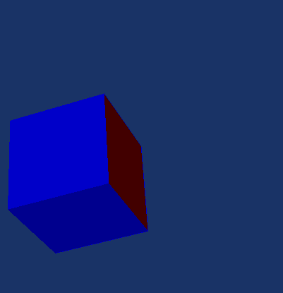
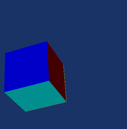
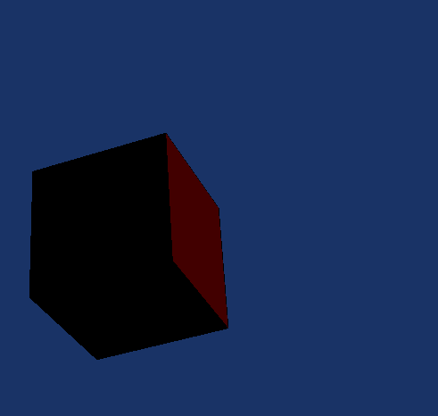
5. Executing this modified pipeline should generate the tomato-colored cube as shown here in the right-hand panel of the "Minimalistic Cube" figure.

Minimalistic Cube: ASCII File & Rendered Image

# vtk DataFile Version 2.0 
Cube example 
ASCII 
DATASET POLYDATA 
POINTS 8 float 
0.0 0.0 0.0 
1.0 0.0 0.0 
1.0 1.0 0.0 
0.0 1.0 0.0 
0.0 0.0 1.0 
1.0 0.0 1.0
1.0 1.0 1.0
0.0 1.0 1.0
POLYGONS 6 30
4 0 1 2 3 
4 4 5 6 7
4 0 1 5 4
4 2 3 7 6
4 0 4 7 3
4 1 2 6 5

Minimalistic Cube

The sets of numbers used to define the POINTS & POLYGONS of this simple cube are explained here.

6. In an accompanying discussion, we explain how to interpret — and, therefore, also how to modify as desired — the rows and columns of numbers that have been used here to define the POINTS (vertices) and POLYGONS of a simple cube.

7. For fun, use VisTrails' "HTTPFile" module to load each of the following files that provide ASCII data written in VTK's Simple Legacy Format to specify a more intricate multi-polygonal structure. I found these posted on J. Burkardt's FSU website:

Simple Cube
vtk.vtk = (Simple lines spelling out "vtk")
v.vtk = (A 3D version of the letter "v")
t.vtk = (A 3D version of the letter "t")
k.vtk = (A 3D version of the letter "k")

Reading Cube Model from a Local File

You will be afforded a much greater degree of design flexibility if, rather than asking VisTrails to download the file from a web site, you create a local file (on the same computer that you are using to run VisTrails) that contains the POINTS and POLYGONS defining the cube and instruct VisTrails to read the information from that local file. Initially, the file need only contain the 20 lines of ASCII text that are displayed in the left-hand panel of the above "Minimalistic Cube" figure.

1. Create a new file on your computer and either (a) type the 20 lines of ASCII text into the file by hand, or (b) copy the ASCII text from the "SimpleCube_Step01.vtk" file provided at the above-referenced web site and paste that information into your new file.

Be very careful doing this because the "vtkPolyDataReader" module in VisTrails is very picky. In order to guarantee success, the file should be formatted in precisely the manner used here, that is, using the Simple Legacy Format described in §15.3 (pp. 324-336) of the VTK User's Guide.
For the purposes of this tutorial exercise, when you save the file, name it TestCube01.txt; to comply with the Simple Legacy Format standards, be sure to save it as a "text only" file.

2. Point the "vtkPolyDataReader" module to this new file:

Disconnect (and, if desired, delete) the "HTTPFile" module from the VisTrails pipeline.
Click on (i.e., highlight) the "vtkPolyDataReader" module in the pipeline, then drag the "SetFile" method into the "Set Methods" segment of the VisTrails Builder Window.
A small folder icon will appear immediately to the right of the newly created "File" text window; click on this icon, then march through your computer's file folders to find your newly created TestCube01.txt file.

3. Executing this modified pipeline should, once again, generate the tomato-colored cube as shown in the right-hand panel of the above "Minimalistic Cube" figure.

CAUTION (from J. E. Tohline): This simple step caused me considerable grief when I was first trying to understand how to enlist VisTrails in my research activities. I already understood how to numerically define the vertices and polygons of a desired wireframe model for, say, a three-dimensional isodensity contour of one of my group's astrophysical fluid flow simulations. But I had difficulty figuring out how to write that information to a file in a format that VisTrails could understand.

In an effort to minimize typing mistakes, I searched for a web site from which I could copy-and-paste the entire "Cube example" provided on pp. 331-332 of the VTK User's Guide. I discovered that the entire "VTK File Formats" discussion from the VTK User's Guide was posted on a Caltech website, but my copy-and-paste operation introduced quite a few additional white spaces — and deleted others — at locations within the text file that violated rules established within the context of the Simple Legacy Format. As a result, the "vtkPolyDataReader" module misinterpreted the information and, as a consequence, the VisTrails pipeline failed to generate an image. This was difficult to debug because I had no idea whether the data file was corrupted or whether I had screwed up the design of the VisTrails pipeline.

If you are able to successfully generate the tomato-colored cube by using the "HTTPFile" module to download the "SimpleCube_step01.vtk" file from the above-referenced web site but you are not immediately able to generate the same tomato-colored cube by calling upon the "vtkPolyDataReader" module to directly access your newly created text file, it is very likely that your file does not strictly conform to the Simple Legacy Format. Check to make sure that the file you have created does not have hidden formatting instructions, such as unwanted forced line feeds.

4. After you have successfully generated the tomato-colored cube by reading the cube model in from a local file, you should change the extension of the file name from ".txt" to ".vtk". This should be done because (see the opening paragraph of the "Dataset Format" discussion on p. 326 of the VTK User's Guide), by convention VTK files written in Simple Legacy Format use the .vtk file extension regardless of the dataset type contained in the file. After making this change, repeat steps #2 and #3 to make sure you can still generate the minimalistic cube.

Constructing a More Sophisticated Cube

Now comes the fun part. Let's add some more information to the input model data file and, in addition, activate some more methods associated with the various VisTrails modules in order to generate more sophisticated cubes.

Default Color Table

Specifying Colors of Cell Faces Using a Default Color Table

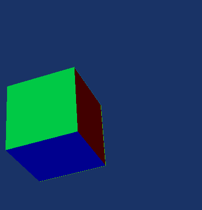
Tutorial Task: Assign a separate scalar value to each of the six faces of the cube, then color the faces differently, in accordance with their assigned scalar values. Continuing to adhere to the Simple Legacy Format, this can be accomplished by adding nine lines of ASCII text to the text file that was created, above, to draw a minimalistic cube. Each column of the following table presents (top of the column) an example of this additional ASCII text, along with (bottom of the column) the resulting cube image, as rendered by VisTrails.

Example A

Example B

Example C

# vtk DataFile Version 2.0
Cube example
ASCII
DATASET POLYDATA
POINTS 8 float
0.0 0.0 0.0
1.0 0.0 0.0
1.0 1.0 0.0
0.0 1.0 0.0
0.0 0.0 1.0
1.0 0.0 1.0
1.0 1.0 1.0
0.0 1.0 1.0
POLYGONS 6 30
4 0 1 2 3
4 4 5 6 7
4 0 1 5 4
4 2 3 7 6
4 0 4 7 3
4 1 2 6 5

CELL_DATA 6
SCALARS cell_scalars float 1
LOOKUP_TABLE default
0.0
0.2
0.4
0.6
0.8
1.0

(same first 20 lines of text)
.
.
.



.
.
.



.
.
.





CELL_DATA 6
SCALARS cell_scalars float 1
LOOKUP_TABLE default
0.0
0.1
0.2
0.3
0.4
0.5

(same first 20 lines of text)
.
.
.



.
.
.



.
.
.





CELL_DATA 6
SCALARS cell_scalars int 1
LOOKUP_TABLE default
0
1
2
3
4
5

Corresponding Rendering of Cube by VisTrails

General Explanation:

"CELL_DATA 6" means that the subsequent numerical values should be assigned, in sequence, to each of the 6 polygonal (square) faces of the cube.
"SCALARS cell_scalars float 1" (see Examples A & B) means that, in each case, the assigned numerical value will be a floating-point number; "SCALARS cell_scalars int 1" (see Example C) means that the assigned numerical value will be an integer number. As necessary, the name "cell_scalars" will be used to reference this assigned set of scalar values. In principle, up to four separate sets of scalar values can be assigned to the faces of the cube (see the discussion associated with the parameter numComp on p. 329 of the VTK User's Guide); the "1" at the end of this line of text indicates that the values associated with the name "cell_scalars" will be referenced as the first scalar component; it is optional if there is only one scalar component.
"LOOKUP_TABLE default" means that the color that is assigned to each face will be determined by correlating the scalar value assigned to each face with the scalar values assigned to the standard rainbow of colors as defined by VTK's default lookup color table.

Example A:

The six assigned floating-point numbers range from 0.0 to 1.0, in increments of 0.2. By inspection, it appears as though VTK's default color table spreads the rainbow of (RGB) colors across this same interval, with 0.0 being assigned to red and 1.0 being assigned to blue. It is therefore not surprising that the three initially visible faces of the rendered cube are red, green, and blue. The colors of the other three faces of the cube are revealed by using the computer mouse to spin the VisTrails spreadsheet rendering of the cube.

Example B:

The six assigned floating-point numbers range from 0.0 to 0.5, in increments of 0.1. Because three of the assigned scalar values (0.0, 0.2, and 0.4) match values assigned in Example A, three of the faces of this cube should have the same colors as three of the faces of the Example A cube, but not necessarily the same cube face in both examples. Also, none of the faces is blue because the assigned scalar values all lie well below 1.0.

Example C:

The six assigned integer numbers range from 0 to 5, in increments of 1. One face — the one whose assigned scalar value is zero — is colored red; all five other faces are colored blue because the color table does not extend beyond 1.0 and VTK's default coloring rule (see further elaboration, below) is to peg scalar values at one (i.e., blue) if their assigned values are greater than unity.

Comment#1 (by J. E. Tohline): Notice that, once a set of scalar values has been assigned to cell faces, the colors provided by the default LOOKUP_TABLE override the "tomato" color that is specified by the "vtkProperty" module of the VisTrails pipeline. The default "tomato" color can be retrieved without modifying the new input datafile by clicking on (i.e., selecting) the "vtkPolyDataMapper" module in the VisTrails pipeline, dragging the "ScalarVisibilityOff" method into the "Set Methods" segment of the VisTrials Builder Window, then reexecuting the pipeline.

Comment#2 (by J. E. Tohline): Example C, shown here, adopts the same CELL_DATA scalar values that appear in the simple "cube example" presented in §15.3 (see the top of p. 332) of the VTK User's Guide. In my opinion, this was a very odd choice to make if its purpose was to help students understand how the VTK and/or VisTrails machinery works. I, for one, was pretty sure I was still doing something wrong when I was finally able to read the "cube example" file into the VisTrails "vtkPolyDataReader," because most of the faces of the cube were painted the same color (blue) whereas I was expecting them all to have different, illustrative colors.

Deciphering VTK's default Lookup Table

While color values that are prescribed by VTK's default lookup table have been used in the three example ASCII files just discussed — Examples A, B, and C — the code that VTK uses to map scalar values to specific colors has not been explicitly provided. When I began trying to understand, for myself, how color specification is handled in VTK, I was unable to locate a reference that spells out what the properties are of the default lookup table. By experimentation I discovered that a simple lookup table that comes close to mimicking the default one is as follows:

LOOKUP_TABLE my_table 6
1.0 0.0 0.0 1.0
1.0 1.0 0.0 1.0
0.0 1.0 0.0 1.0
0.0 1.0 0.0 1.0
0.0 1.0 1.0 1.0
0.0 0.0 1.0 1.0

Eventually I discovered documentation that defines the default settings for VTK's color maps. In §6.6 of Schroeder, Martin, & Lorensen (2006) (see specifically the subsection titled Color Maps on p. 196), we are told the default settings are established via a specification of HSV (Hue-Saturation-Value) rather than via an rgb specification. The default settings are: HueRange (0, 2/3); SaturationRange (1,1); and ValueRange (1,1). This terminology is explained in an accompanying presentation.

Specifying Colors of Cell Faces via a User-defined Color Table

Now, suppose you don't like the colors that are assigned to each of the six faces of the cube by VTK's default color table. You can assign a different set of colors by explicitly defining your own "LOOKUP_TABLE." To illustrate how this is done, we have added nine additional lines of ASCII text to the input data files shown in Example D and Example E, below. In both cases, we have inserted the LOOKUP_TABLE that has been provided as part of the "simple cube" example that is provided on pp. 331-332 of the VTK User's Guide.

LOOKUP_TABLE Example in Simple Legacy Format

Example A

Example D

Example E

Color Code

# vtk DataFile Version 2.0
Cube example
ASCII
DATASET POLYDATA
POINTS 8 float
0.0 0.0 0.0
1.0 0.0 0.0
1.0 1.0 0.0
0.0 1.0 0.0
0.0 0.0 1.0
1.0 0.0 1.0
1.0 1.0 1.0
0.0 1.0 1.0
POLYGONS 6 30
4 0 1 2 3
4 4 5 6 7
4 0 1 5 4
4 2 3 7 6
4 0 4 7 3
4 1 2 6 5

CELL_DATA 6
SCALARS cell_scalars float 1
LOOKUP_TABLE default
0.0
0.2
0.4
0.6
0.8
1.0

(same first 20 lines of text)
.
.
.



.
.
.


CELL_DATA 6
SCALARS cell_scalars float 1
LOOKUP_TABLE my_table
0.0
0.1
0.2
0.3
0.4
0.5
LOOKUP_TABLE my_table 8
0.0 0.0 0.0 1.0
1.0 0.0 0.0 1.0
0.0 1.0 0.0 1.0
1.0 1.0 0.0 1.0
0.0 0.0 1.0 1.0
1.0 0.0 1.0 1.0
0.0 1.0 1.0 1.0
1.0 1.0 1.0 1.0

(same first 20 lines of text)
.
.
.



.
.
.


CELL_DATA 6
SCALARS cell_scalars float 1
LOOKUP_TABLE my_table
0.14286
0.28571
0.42857
0.57143
0.71429
0.85714
LOOKUP_TABLE my_table 8
0.0 0.0 0.0 1.0
1.0 0.0 0.0 1.0
0.0 1.0 0.0 1.0
1.0 1.0 0.0 1.0
0.0 0.0 1.0 1.0
1.0 0.0 1.0 1.0
0.0 1.0 1.0 1.0
1.0 1.0 1.0 1.0

R	G	B	Result	HEX
0.0	0.0	0.0	black	000000
1.0	0.0	0.0	red	FF0000
0.0	1.0	0.0	green	00FF00
1.0	1.0	0.0	yellow	FFFF00
0.0	0.0	1.0	blue	0000FF
1.0	0.0	1.0	magenta	FF00FF
0.0	1.0	1.0	cyan	00FFFF
1.0	1.0	1.0	white	FFFFFF

See also Figure 3-4 (p. 38) of
Schroeder, Martin, & Lorensen (2006)

Corresponding Rendering of Cube by VisTrails

General Explanation:

The VTK User's Guide (see bottom of p. 329), explains the construction of the Simple Legacy Format LOOKUP_TABLE as follows:

LOOKUP_TABLE tableName size
<math>r_0 ~g_0 ~b_0 ~\alpha_0</math>

<math>r_1 ~g_1 ~b_1 ~\alpha_1</math>

…

<math>r_{size-1} ~g_{size-1} ~b_{size-1} ~\alpha_{size-1}</math>

The tableName field is a character string (without imbedded white space) used to identify the lookup table. This label is used by the VTK reader to extract a specific table.

Each entry in the lookup table is a rgba (red-green-blue-alpha) array (alpha is opacity where alpha = 0 is transparent). If the file format is ASCII, the lookup table values must be float values between (0,1).

Notice that the LOOKUP_TABLE that has been added to the ASCII input data file in Examples D and E has tableName = my_table and has size = 8, that is, it contains eight distinct rgba colors — each row of numbers specifies a distinct color and, in this case, they all have the same transparency, <math>~\alpha=1.0</math> (i.e., completely opaque). The "color code" table that has been provided to the right of Example E shows what color results from each of the eight assigned RGB triplets; the equivalent hexadecimal representation is provided for each color as well.
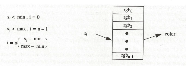
As is explained in §6.2 of Schroeder, Martin, & Lorensen (2006), the mapping of scalar values to the color table proceeds as follows:

Mapping Scalar Values to the Color Lookup Table
[copied from Schroeder, Martin, & Lorensen (2006)]

As illustrated above, in the first bulleted comment under General Explanation, "the lookup table holds an array of colors (e.g., red, green, blue components or other comparable representations). Associated with the table is a minimum and maximum scalar range (min, max) into which the scalar values are mapped. Scalar values greater than the maximum range are clamped to the maximum color, scalar values less than the minimum range are clamped to the minimum color value. Then, for each scalar value <math>~s_i</math>, the index <math>~i</math> into the color table with <math>~n</math> entries (and 0-offset) is given by" the figure shown here.

Example A: (Identical to Example A shown earlier)

The six scalar (floating-point) values that have been assigned to the six faces of the cube range from 0.0 to 1.0, in increments of 0.2. Presumably, VTK's default color table spreads the rainbow of (RGB) colors across this same interval, with 0.0 being assigned to red and 1.0 being assigned to blue.

Example D:

As in Example B shown earlier, the six assigned floating-point scalars range from 0.0 to 0.5, in increments of 0.1. But now the second line of text following CELL_DATA 6 explicitly tells the VTK reader to refer to the user-provided "LOOKUP_TABLE" called my_table when assigning a color to each of the six scalar values.
As I understand it, VTK will assign the first of the eight colors (black) to a scalar value of 0.0 and it will assign the last of the eight colors (white) to a scalar value of 1.0; the other six colors get mapped in linear proportion to scalar values that fall between 0.0 and 1.0.
(This comment will make more sense after studying Example E.) It appears as though the scalar values are rounded down before a color assignment is made — and it looks like there is no interpolation between colors: A complete examination of the cube that is generated by VisTrails from the Example D input file reveals that the two sides labeled as polygons #0 and #1 are painted black, presumably because they both have been assigned scalar values < 1/7 = 0.14286; polygon #2 is painted red, presumably because it has been assigned a scalar value lying between 1/7 and 2/7; polygon #3 is painted green, presumably because its scalar value lies between 2/7 and 3/7; etc. None of the faces of the cube have been colored magenta, cyan, or white, presumably because their assigned scalar values are all less than 5/7 = 0.57143.

Example E:

This is the same as Example D, except that six new scalar values have been assigned to the six polygons that define the faces of the cube.
With the intent of avoiding the first and last colors (black and white) in the lookup table but assigning one each of the other six colors to each of the six cube faces, we have assigned scalar values that are an integer number times 1/7, that is, the values: 1/7, 2/7, 3/7, 4/7, 5/7, and 6/7. This was done based on the assumption, as stated earlier in connection with Example D, that black gets mapped to a scalar value of 0.0 (or less), white gets mapped to a scalar value of 1.0 (or greater), while "the other six colors get mapped in linear proportion to scalar values that fall between 0.0 and 1.0."
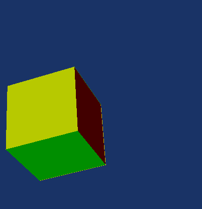
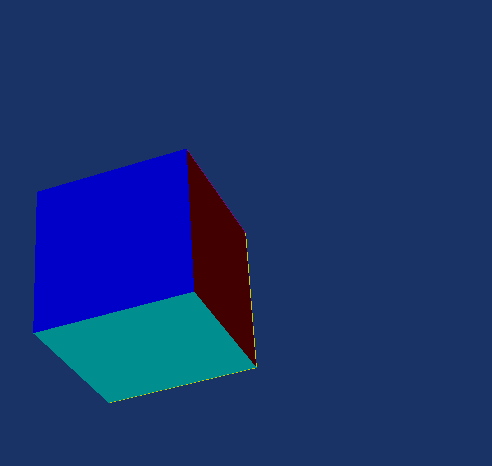
Success! The rendered cube that initially appears in the VisTrails spreadsheet (see the image at the bottom of the "Example E" figure column, above) shows three sides of the cube colored red, blue, and cyan corresponding to, respectively, polygons #0, #3, and #5. Spinning the cube will allow you to view all three of the other lookup table colors: green (polygon #1), yellow (polygon #2), and magenta (polygon #4).

As part of this tutorial, you are now encouraged to explore how the coloring of the faces of this "simple cube" are altered when different scalar values are assigned or when different triplets of RGB colors are specified in the user-provided LOOKUP_TABLE. For example: try assigning scalar values that are greater than unity or less than zero; try using fractional values (that is, not just 1.0 or 0.0) for the R, G, and/or B table specifications; and try designing a larger color table, say, one that contains a dozen or more different colors (don't forget to change the value of the size parameter in the header of the LOOKUP_TABLE).

Other Knobs to Twist

Cheetsheet
Module:	Method Action:	Result
vtkPolyDataReader	SetLookupTableName = my_table	my_table^†
vtkPolyDataReader	SetLookupTableName = default	VTK's default hue-based color table
vtkPolyDataReader	SetLookupTableName = default	Color table provided by vtkLookupTable module, if one hooked into vtkPolyDataMapper
vtkPolyDataMapper	ScalarVisibilityOff	Color defined by vtkProperty module
vtkProperty	SetRepresentationToWireframe	Rendered as wireframe only
^†Table obtained from Simple Legacy Formatted input file

Switch Between Different Color Tables:

When using the input data file associated with Example E, the six faces of the cube will be colored according to the values assigned by the user to the "my_table" LOOKUP_TABLE. You can straightforwardly switch to VTK's "default" color table without further modifying the input data file by clicking on (i.e., selecting) the "vtkPolyDataReader" module in the VisTrails pipeline, dragging the "SetLookupTableName" method into the "Set Methods" segment of the VisTrails Builder Window, typing the string "default" into the provided window, then reexecuting the pipeline. (You can switch back to the user-provided color table by typing in the string "my_table", then reexecuting the pipeline.)
You can also revert back to the tomato-colored cube (or whatever color is specified inside the "vtkProperty" module) by clicking on the "vtkPolyDataMapper" module in the VisTrails pipeline, dragging the "ScalarVisibilityOff" method into the "Set Methods" segment of the BisTrails Builder Window, then reexecuting the pipeline.

Transparency:

The fourth floating-point number <math>~(\alpha)</math> that appears in each row of the color LOOKUP_TABLE allows you to assign a transparency (as well as a specific color) to each polygon that has the relevant scalar value. Experiment with changing this number from 1.0 (opaque) to 0.0 (fully transparent, or any fractional value in between (partial transparency).

Use vtkLookupTable Module:

You can construct a wide range of different color Lookup Tables by adding the "vtkLookupTable" module to the VisTrails pipeline. In an accompanying presentation, we explain and illustrate how this is done.

Wireframe:

If, at any time, you want to render only the underlying wireframe structure of your three-dimensional configuration, simply activate the '"SetRepresentationToWireframe" method inside the "vtkProperty" module.

Assigning NORMALS to POLYGONS

Annotated Cube

In an accompanying presentation (which includes a larger image of the Annotated Cube shown here, on the right), we explain how VTK's Simple Legacy Format reader identifies (and internally catalogs) the unit vector that points perpendicular to — and, hence, that defines the normal of — each POLYGON. Here, after highlighting the key points of this more detailed presentation, we illustrate how different definitions of the polygon NORMALS can be specified by inserting additional lines of data into the input data file.

Default Assignment:

Take POLYGON "1" as an example, for which the defining line of input data is "4 4 5 6 7." Adhering to the right-hand rule, VTK understands that, as POINTS 4, 5, 6, & 7 are connected in that order, the perimeter of the four-sided polygon is being traversed in a counter-clockwise direction. Accordingly, by default, VTK records (internally) that the unit vector that is normal to POLYGON "1" points in the <math>~(x,y,z) = (0,0,1)</math> direction.
In the spirit of a tutorial, we recommend that the reader carefully examine the sets of integers that appear immediately following the heading "POLYGONS 6 30" in the above example input data file(s) and answer the following question: In what default direction will VTK determine that the normal to each of the cube's other five POLYGONS points? In other words, fill in the blank spaces in the following table.

POLYGON Number	Direction that unit normal points
POLYGON Number	<math>~x</math>	<math>~y</math>	<math>~z</math>
0
1	0	0	+1
2
3
4
5

Continuing to adhere to the Simple Legacy Format, the user can specify what unit vector normal gets assigned to each POLYGON. If <math>~N_\mathrm{poly}</math> POLYGONS have been defined, then this can be accomplished by inserting an additional <math>~(N_\mathrm{poly} + 1)</math> lines of text to the input data file immediately after scalar values have been assigned to each POLYGON. The top segment of each column of the following table presents an input data file that is identical to Example E, shown above, except 7 additional lines of text have been inserted, beginning with a header line of text that reads, "NORMALS cell_normals float." Only the specified NORMALS change across these three examples, F, G, & H; as before, the image of the cube that is rendered by VisTrails in each case is shown at the bottom of the respective table column.

Example F

Example G

Example H

(same first 20 lines of text)
.
.
.

CELL_DATA 6
SCALARS cell_scalars float 1
LOOKUP_TABLE my_table
0.14286
0.28571
0.42857
0.57143
0.71429
0.85714
NORMALS cell_normals float
0 0 -1
0 0 1
0 -1 0
0 1 0
-1 0 0
1 0 0
LOOKUP_TABLE my_table 8
0.0 0.0 0.0 1.0
1.0 0.0 0.0 1.0
0.0 1.0 0.0 1.0
1.0 1.0 0.0 1.0
0.0 0.0 1.0 1.0
1.0 0.0 1.0 1.0
0.0 1.0 1.0 1.0
1.0 1.0 1.0 1.0

(same first 20 lines of text)
.
.
.

CELL_DATA 6
SCALARS cell_scalars float 1
LOOKUP_TABLE my_table
0.14286
0.28571
0.42857
0.57143
0.71429
0.85714
NORMALS cell_normals float
0 0 1
0 0 1
0 -1 0
0 1 0
-1 0 0
1 0 0
LOOKUP_TABLE my_table 8
0.0 0.0 0.0 1.0
1.0 0.0 0.0 1.0
0.0 1.0 0.0 1.0
1.0 1.0 0.0 1.0
0.0 0.0 1.0 1.0
1.0 0.0 1.0 1.0
0.0 1.0 1.0 1.0
1.0 1.0 1.0 1.0

(same first 20 lines of text)
.
.
.

CELL_DATA 6
SCALARS cell_scalars float 1
LOOKUP_TABLE my_table
0.14286
0.28571
0.42857
0.57143
0.71429
0.85714
NORMALS cell_normals float
0 0 1
0 0 -1
0 1 0
0 -1 0
1 0 0
-1 0 0
LOOKUP_TABLE my_table 8
0.0 0.0 0.0 1.0
1.0 0.0 0.0 1.0
0.0 1.0 0.0 1.0
1.0 1.0 0.0 1.0
0.0 0.0 1.0 1.0
1.0 0.0 1.0 1.0
0.0 1.0 1.0 1.0
1.0 1.0 1.0 1.0

Corresponding Rendering of Cube by VisTrails

General Explanation:

"NORMALS cell_normals float" means that the subsequent six lines of data should be assigned, in sequence, to each of the 6 polygonal (square) faces of the cube; the name "cell_normals" should be assigned to this set of data; and the VTK reader should expect the data to be provided as a set of space-delimited floating point numbers.
Each line of data should contain three numbers to specify the orientation of the unit vector that is normal to the associated POLYGON. In order to determine the unit vector's orientation, the VTK reader assumes that the base of the unit vector is located at the origin of the coordinate system and it will interpret the numbers as identifying the x, y, z coordinates of the other end — that is, the pointed tip — of the unit vector. Hence <math>~(x,y,z) = (0,0,1)</math>, as has been specified for POLYGON "1" in Examples F & G, means that the NORMAL vector assigned to POLYGON "1" points in the plus z direction.

Example F:

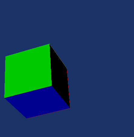
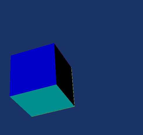
The six lines of coordinate triplets that have been specified in this example contain precisely the same values as the simple "Cube example" that is presented in §15.3 (see the top of p. 332) of the VTK User's Guide. The rendered image is identical to the image that was rendered, above, in Example E — in which the NORMALS were not explicitly specified — except that POLYGON "0" is colored black instead of red. (Spinning the cube around will show that the other five cube faces have the same colors as in Example E.)

More Complete Understanding: (Disclaimer … Because I am not an expert in the design of VTK, I am not sure that the following statements are precisely correct. But they give a pretty good idea of what is accomplished via the specification of NORMALS.)

Especially when a group of POLYGONS is assembled to construct the surface of a 3D structure, VTK needs to know which side of each POLYGON "faces out" and which side "faces in" before it can provide a proper visual rendering of the configuration.
Upon inspection, it is clear that the six sets of coordinate triplets that have been specified in Example F (copied directly from the simple "Cube example" in the VTK User's Guide) all define NORMALS that are pointing "out" of the cube.
My initial assumption was that VTK routines would paint all of the "outward facing" sides of the POLYGONS the color corresponding to their scalar values, but that it may leave uncolored any sides that are "inward facing." I was therefore surprised to discover that the VisTrails rendering that resulted from Example F has one uncolored side — in the rendered image, POLYGON "0" (i.e., the polygon lying in the x-y plane) is black instead of red.
After carefully reanalyzing the information contained in the input data file I realized that, given the definitions of the six POLYGONS provided by the input data file (as copied from the simple "Cube example" in the VTK User's Guide), VTK's default assignment of unit vector normals should be as follows:

VTK's Default Assignment of Unit Vector Normals:
 0  0 +1
 0  0 +1
 0 -1  0
 0 +1  0
-1  0  0
+1  0  0

This is the set of six triplet values that should be entered into the above table to answer the tutorial quiz question: In what default direction will VTK determine that the normal to each of the cube's other five POLYGONS points? It differs from the set of cell_normals that we have explicitly inserted into Example F, above, in one very important way: The cell normal that has been assigned to POLYGON "0" in Example F is <math>~(x,y,z) = (0,0,-1)</math> whereas, given the order in which the POINTS are specified when POLYGON "0" is defined in the input data file (4 0 1 2 3) and an adherence to the right-hand rule, the default direction that would be assigned by VTK is <math>~(x,y,z) = (0,0,+1)</math>.

Comment#3 (by J. E. Tohline): Initially, it wasn't obvious to me why POLYGON "0" was black. Because all of the "cell_normals" NORMALS that are explicitly specified in the Example F input data file point "out," I expected all six faces of the cube to be colored as shown in Example E. It took me a while to deduce that the default normal that VTK assigned to POLYGON "0" was <math>~(0,0,+1)</math> and pointed "into," rather than "out of," the cube. POLYGON "0" was painted black because the explicitly specified NORMAL in Example F pointed in the opposite direction to this default normal. In my opinion, this was an odd set of numbers for the VTK User's Guide to provide in order to illustrate how to specify NORMALS in the simple "Cube example."

Example G:

If I was correct in explaining why POLYGON "0" was rendered black in Example F, then it should be possible to return POLYGON "0" to a red color by doing one of two things: (1) Flip the explicitly specified NORMAL to <math>~(0,0,+1)</math>, putting it in alignment with the normal's default specification; or (2) redefine POLYGON "0" by reversing the order in which its four POINTS are connected so that, according to the right-hand rule convention, the default normal would point "out of" rather than "into" the cube. The first of these two adjustments was made in Example G. Only one line of data in the Example G input file is different from the Example F input file: the NORMAL specified for POLYGON "0" is <math>~(0,0,1)</math> instead of <math>~(0,0,-1)</math>. As predicted, the VisTrails pipeline colored POLYGON "0" red instead of black.

Example H:

Example H differs from Example F in that the direction of all six of the specified normals is reversed; that is, in Example H, all of the explicitly specified normals point "into" rather than "out of" the cube. As expected, the resulting rendered image has one red side (POLYGON "0"), while the other five cell faces are black — indicating that, for each face, the explicitly specified NORMAL and the default normal point in opposite directions.

XML-Formatted Input

Overview

As is explained in §15.3 (see the bottom of p. 336) of the VTK User's Guide, authored and published by Kitware, Inc., VTK (and VisTrails) also supplies Readers that accept XML-formatted input data. An example XML-formatted data file is shown immediately following this paragraph; it also can be obtained at the following website:

http://www.phys.lsu.edu/~tohline/vistrails/datafiles/XMLformattedSimpleCube.vtp

The information provided in this 34-line ASCII file describes exactly the same "Simple Cube" model that was presented above in Simple Legacy Format as Example G. It is also similar — but not identical — to the example XML-formatted data file presented on p. 346 of the VTK User's Guide.

<?xml version="1.0"?>
<VTKFile type="PolyData" version="0.1" byte_order="LittleEndian">
  <PolyData>
    <Piece NumberOfPoints="8" NumberOfPolys="6">
      <CellData Scalars="cell_scalars" Normals="cell_normals">
        <DataArray type="Float32" Name="cell_scalars" format="ascii">
          0.14286 0.28571 0.42857
          0.57143 0.71429 0.85714
        </DataArray>
        <DataArray type="Float32" Name="cell_normals" NumberOfComponents="3" format="ascii">
          0 0 1 0 0 1 0 -1 0 0 1 0 -1 0 0 1 0 0
        </DataArray>
      </CellData>
      <Points>
        <DataArray type="Float32" NumberOfComponents="3" format="ascii">
          0 0 0 1 0 0
          1 1 0 0 1 0
          0 0 1 1 0 1
          1 1 1 0 1 1
        </DataArray>
      </Points>
      <Polys>
        <DataArray type="Int32" Name="connectivity" format="ascii">
          0 1 2 3  4 5 6 7
          0 1 5 4  2 3 7 6
          0 4 7 3  1 2 6 5
        </DataArray>
        <DataArray type="Int32" Name="offsets" format="ascii">
          4 8 12 16 20 24
        </DataArray>
      </Polys>
    </Piece>
  </PolyData>
</VTKFile>

General Explanation:

The "Piece" of the "PolyData" being described in this file contains 8 points and 6 polygons (polys). The substantive information is provided by "Data Arrays" located within three subsections of the file: CellData, Points, and Polys.
Points: This DataArray provides the same information as the POINTS subsection of a Simple Legacy Formatted data file, that is, it specifies the <math>~(x, y, z)</math> coordinates of the eight points (vertices) of our simple cube. The header of this DataArray tells the VTK Reader that it should read 3 numbers (the coordinates) at a time, and that the (space-delimited) data should be read as 32-bit floating-point numbers. The Reader will expect this DataArray to contain (NumberOfPoints x NumberOfComponents =) 24 separate floating-point numbers.
Polys: In combination with one another, the two DataArrays found between the Polys metatags provide the same information as the POLYGONS subsection of a Simple Legacy Formatted data file. The first DataArray, whose Name is "connectivity," identifies the group of POINTS that should be connected to define the complete perimeter of each face of the cube; the second DataArray, whose Name is "offsets," tells the Reader how many integers in the "connectivity" array should be skipped in order to begin defining each subsequent polygon. In other words, the number of POINTS that define the perimeter of each polygon — in this case, 4 for every polygon — is given by the difference between successive offsets.
CellData: The first DataArray, whose name is "cell_scalars," assigns a scalar value to each polygon, i.e., to each face of the cube; the Reader will expect this DataArray to contain (NumberOfPolys =) 6 separate 32-bit floating-point numbers. The second DataArray, whose name is "cell_normals," specifies the <math>~(x, y, z)</math> coordinates of the tip of the unit vector that defines the NORMAL to the surface of each polygon, as explained in the discussion, above; the Reader will expect this DataArray to contain (NumberOfPolys x NumberOfComponents =) 18 separate 32-bit floating-point numbers.

Pipeline02

XMLPolyDataReader:

The figure labeled "Pipeline01" near the top of this page, shows the VisTrails pipeline that we used to construct and render a simple cube based on a web-accessible input file that provides data in a Simple Legacy Format. That input data was fed into the VisTrails pipeline using the vtkPolyDataReader module. As is illustrated by the "Pipeline02" figure, shown here on the right, the equivalent XML-formatted data file — which, as noted immediately above, is accessible on the web as a file named XMLformattedSimpleCube.vtp — can be fed into the VisTrails pipeline using the vtkXMLPolyDataReader module.

No Color Table: As far as I have been able to ascertain, XML-formatted data files cannot be used to define LOOKUP_TABLEs — that is, color tables. Hence, as illustrated in the "Pipeline02" figure shown here on the right, a vtkLookupTable module must be inserted into the VisTrails pipeline if the user wants to define the color table.

Comment Lines and Deleting XML Pieces

Two major advantages of XML-formatted input data files is the ability to segment the data — and rendered elements of a scene — into separate Pieces and, then, the ability to "comment out" one or more of these pieces when you want to simplify the scene. The following ASCII data file illustrates how the Simple Cube can be subdivided into a pair of 3-sided figures and how, by simply inserting or deleting a comment line, the two Pieces can be rendered together or separately.

<?xml version="1.0"?>
<VTKFile type="PolyData" version="0.1" byte_order="LittleEndian" compressor="vtkZLibDataCompressor">
  <PolyData>
<!-- This is three of the sides of the cube -->
    <Piece NumberOfPoints="8" NumberOfPolys="3">
      <CellData Scalars="temperature" Normals="cell_normals">
        <DataArray type="Float32" Name="temperature" format="ascii">
          0.14286 0.28571 0.42857
        </DataArray>
        <DataArray type="Int32" Name="cell_normals" NumberOfComponents="3" format="ascii">
          0 0 1  0 0 1  0 -1 0
        </DataArray>
      </CellData>
      <Points>
        <DataArray type="Float32" NumberOfComponents="3" format="ascii">
          0 0 0 1 0 0
          1 1 0 0 1 0
          0 0 1 1 0 1
          1 1 1 0 1 1
        </DataArray>
      </Points>
      <Polys>
        <DataArray type="Int32" Name="connectivity" format="ascii">
          0 1 2 3   4 5 6 7   0 1 5 4
        </DataArray>
        <DataArray type="Int32" Name="offsets" format="ascii">
          4 8 12
        </DataArray>
      </Polys>
    </Piece>
<!-- This is the other three sides of the cube
    <Piece NumberOfPoints="8" NumberOfPolys="3">
      <CellData Scalars="temperature" Normals="cell_normals">
        <DataArray type="Float32" Name="temperature" format="ascii">
          0.57143 0.71429 0.85714
        </DataArray>
        <DataArray type="Int32" Name="cell_normals" NumberOfComponents="3" format="ascii">
          0 1 0  -1 0 0  1 0 0
        </DataArray>
      </CellData>
      <Points>
        <DataArray type="Float32" NumberOfComponents="3" format="ascii">
          0 0 0 1 0 0
          1 1 0 0 1 0
          0 0 1 1 0 1
          1 1 1 0 1 1
        </DataArray>
      </Points>
      <Polys>
        <DataArray type="Int32" Name="connectivity" format="ascii">
          2 3 7 6    0 4 7 3   1 2 6 5
        </DataArray>
        <DataArray type="Int32" Name="offsets" format="ascii">
          4 8 12
        </DataArray>
      </Polys>
    </Piece>
-->
  </PolyData>
</VTKFile>

General Explanation:

The fourth line of the above ASCII data file is a single, standard XML-formatted comment line — see the explanation provided, for example, on the Wikipedia page that explains XML comment tags. By XML convention, it begins with the string "<math>~< !--</math>" and ends with the string "<math>~--></math>". The same beginning and ending strings also appear, respectively, as lines 31 and 58 in the data file. In the first case, because the two strings appear on the same line of the file, they simply serve to encapsulate a short comment. In the second case, all of the ASCII text that falls between lines 31 and 58 are considered part of the "comment" and therefore the second Piece of the cube is ignored by the XMLPolyDataReader. As presented here, this input data file will generate only three sides of the cube. The entire cube will be rendered if line 58 is deleted and the string "<math>~--></math>" is added to the end of line 31.

WarpScalar

In an effort to figure out how to display the free-energy surface of self-gravitating fluid systems, I decided to see if I could combine what I had just learned about creating (and reading in) XML-formatted data structures with the capabilities of the vtkWarpScalar module. The capabilities of this "warping" module are illustrated by the VisTrails (and VTK) warpComb.vt example:

.../VisTrails/examples/vtk_examples/VisualizationAlgorithms/warpComb.vt

(See also the imageWarp.vt vistrail in the same vtk_examples directory.)

<?xml version="1.0"?>
<VTKFile type="PolyData" version="0.1" byte_order="LittleEndian">
  <PolyData>
    <Piece NumberOfPoints="36" NumberOfPolys="25">
      <CellData Scalars="cell_scalars" Normals="cell_normals">
        <DataArray type="Float32" Name="cell_scalars" format="ascii">
          0.2 0.2 0.2 0.2 0.2
          0.2 0.4 0.6 0.4 0.2
          0.2 0.6 0.8 0.6 0.2
          0.2 0.4 0.6 0.4 0.2
          0.2 0.2 0.2 0.2 0.2
        </DataArray>
        <DataArray type="Float32" Name="cell_normals" NumberOfComponents="3" format="ascii">
          0 0 1   0 0 1   0 0 1   0 0 1  0 0 1
          0 0 1   0 0 1   0 0 1   0 0 1  0 0 1
          0 0 1   0 0 1   0 0 1   0 0 1  0 0 1
          0 0 1   0 0 1   0 0 1   0 0 1  0 0 1
          0 0 1   0 0 1   0 0 1   0 0 1  0 0 1
        </DataArray>
      </CellData>
      <PointData Scalars="colorful" Normals="magnify">
        <DataArray type="Float32" Name="colorful" format="ascii">
          0.2 0.2 0.2 0.2 0.2 0.2
          0.2 0.4 0.6 0.6 0.4 0.2
          0.2 0.6 0.8 0.8 0.6 0.2
          0.2 0.6 0.8 0.8 0.6 0.2
          0.2 0.4 0.6 0.6 0.4 0.2
          0.2 0.2 0.2 0.2 0.2 0.2
        </DataArray>
        <DataArray type="Float32" Name="magnify" NumberOfComponents="3" format="ascii">
          0 0 1   0 0 1   0 0 1   0 0 1  0 0 1  0 0 1
          0 0 1   0 0 1   0 0 1   0 0 1  0 0 1  0 0 1
          0 0 1   0 0 1   0 0 1   0 0 1  0 0 1  0 0 1
          0 0 1   0 0 1   0 0 1   0 0 1  0 0 1  0 0 1
          0 0 1   0 0 1   0 0 1   0 0 1  0 0 1  0 0 1
          0 0 1   0 0 1   0 0 1   0 0 1  0 0 1  0 0 1
        </DataArray>
      </PointData>
      <Points>
        <DataArray type="Float32" NumberOfComponents="3" format="ascii">
         0 0 0 1 0 0 2 0 0 3 0 0 4 0 0 5 0 0
         0 1 0 1 1 0 2 1 0 3 1 0 4 1 0 5 1 0
         0 2 0 1 2 0 2 2 0 3 2 0 4 2 0 5 2 0
         0 3 0 1 3 0 2 3 0 3 3 0 4 3 0 5 3 0
         0 4 0 1 4 0 2 4 0 3 4 0 4 4 0 5 4 0
         0 5 0 1 5 0 2 5 0 3 5 0 4 5 0 5 5 0
        </DataArray>
      </Points>
      <Polys>
        <DataArray type="Int32" Name="connectivity" format="ascii">
           0  1  7  6   1  2  8  7   2  3  9  8   3  4 10  9   4  5 11 10
           6  7 13 12   7  8 14 13   8  9 15 14   9 10 16 15  10 11 17 16
          12 13 19 18  13 14 20 19  14 15 21 20  15 16 22 21  16 17 23 22
          18 19 25 24  19 20 26 25  20 21 27 26  21 22 28 27  22 23 29 28
          24 25 31 30  25 26 32 31  26 27 33 32  27 28 34 33  28 29 35 34
        </DataArray>
        <DataArray type="Int32" Name="offsets" format="ascii">
          4  8 12 16 20 24 28 32 36 40
         44 48 52 56 60 64 68 72 76 80
         84 88 92 96 100
        </DataArray>
      </Polys>
    </Piece>
  </PolyData>
</VTKFile>

1. First, I constructed the new, XML-formatted input data file shown immediately above. The configuration described by this data file has the following key features:

As is detailed in the "Points" DataArray, the configuration has a structured grid containing 6 x 6 = 36 vertices. The z coordinate of all 36 points is zero, which means that the configuration is a plane of zero thickness that is lying in the <math>x-y</math> plane.
The scalar values assigned to these 36 points/vertices are provided in the "PointData" DataArray named "colorful."
As is detailed in the pair of "Polys" DataArrays, the grid points are connected with one another, four at a time, to create 5 x 5 = 25 cells.
The scalar values assigned to these 25 cells are provided in the "CellData" DataArray named "cell_scalars."

2. Next, I read this XML_formatted data file into the VisTrails pipeline discussed above — specifically, the one displayed above as "Pipeline02" — to convince myself that the configuration would be rendered as a multicolored plane.

3. Finally, as is illustrated below in the figure labeled "Pipeline03," I inserted the "vtkWarpScalar" module into the VisTrails pipeline between the XMLPolyData reader and the PolyData Mapper, and activated its SetScaleFactor" method with a value of 2.0. Executing this pipeline generated the image in the upper-right whose caption reads, "Warp (Point Data) Image."

4. The image in the lower-right whose caption reads, "Warp (Cell Data) Image," was generated by activating the SetScalarModeToUseCellData method in the "vtkPolyDataMapper" module.

Pipeline03	Warp (Point Data) Image
	Warp (Cell Data) Image

Other Example Input Files and VisTrails Pipelines

Here we present a number of examples of input data files that we have successfully used to generate useful interactive renderings within VisTrails. The files illustrate VTK's Simple Legacy Format as well as VTK's XML-Formatted file structures. In each case we present the full ascii dataset, the resulting rendered image, and a screen shot of the VisTrails pipeline that was used to generate the image. It is important to notice that, when the dataset format is changed — from, say, POLYDATA to STRUCTURED_POINTS — the corresponding vtk "Mapper" module may need to be changed as well.

Simple Legacy Format

Cube Example G: Uses vtkPolyDataReader & vtkPolyDataMapper
BU (Robert Putnam) Example of Structured Points: Uses vtkStructuredPointsReader & vtkDataSetMapper
Cornell Example of Rectilinear Grid: Uses vtkRectilinearGridReader & vtkDataSetMapper

XML-Formatted

Warped Quilt: Uses vtkXMLPolyDataReader, vtkWarpScalar, & vtkXMLPolyDataMapper
Rectilinear Grid: Uses vtkXMLRectilinearGridReader, vtkWarpScalar, & vtkXMLDataSetMapper
- Warped Quilt (6 x 6 grid)
- Mexican Hat at two different resolutions: (50 x 50 grid) and (10 x 10 grid); the lower resolution example also illustrates how the vtkWarpScalar module handles user-specified Normals.

Related Discussions

Understanding vtk Tools Inside VisTrails
Cube Definition Details
Color Lookup Tables
Robert Putnam's (Boston University) powerpoint tutorial -- includes a Structured_Points example, written in Simple Legacy Format

User:Tohline/vtk/SimpleCubeTutorial

Contents

Simple Cube Tutorial

Getting Started

Minimalistic Cube

Reading Cube Model from a Web Site

Reading Cube Model from a Local File

Constructing a More Sophisticated Cube

Default Color Table

Specifying Colors of Cell Faces Using a Default Color Table

Deciphering VTK's default Lookup Table

Specifying Colors of Cell Faces via a User-defined Color Table

Other Knobs to Twist

Assigning NORMALS to POLYGONS

XML-Formatted Input

Overview

Comment Lines and Deleting XML Pieces

WarpScalar

Other Example Input Files and VisTrails Pipelines

Simple Legacy Format

XML-Formatted

Related Discussions

Navigation menu

Search