Embedded Polytropic Spheres

In a separate discussion we have shown how to determine the structure of isolated polytropic spheres. These are rather idealized stellar structures in which the pressure and density both drop to zero at the surface of the configuration. Here we consider how the equilibrium radius of a polytropic configuration of a given <math>~M</math> and <math>~K_\mathrm{n}</math> is modified when it is embedded in an external medium of pressure <math>~P_e</math>. We will begin by reviewing the general properties of embedded (and truncated) polytropes for a wide range of polytropic indexes, principally summarizing the published descriptions provided by Horedt (1970), by Whitworth (1981) and by Stahler (1983). Then we will focus in more detail on polytropes of index <math>~n</math> = 1 and <math>~n</math> = 5 because their structures can be described by closed-form analytic expressions.

General Properties

Horedt's Presentation

It appears as though Horedt (1970) was the first to draw an analogy between the mass limit that is associated with bounded isothermal spheres — the so-called Bonnor-Ebert spheres — and the limiting mass that can be found in association with equilibrium sequences of embedded polytropes that have polytropic indexes <math>~n > 3</math>. Using a tilde to denote values of parameters at the (truncated) edge of a pressure-bounded polytropic sphere, Horedt (see the bottom of his p. 83) derives the following set of parametric equations relating the configuration's dimensionless radius, <math>~r_a</math>, to a specified dimensionless bounding pressure, <math>~p_a</math>:

<math> ~r_a \equiv \frac{R_\mathrm{eq}}{R_\mathrm{Horedt}} </math>	<math>~=~</math>	<math> \tilde\xi ( -\tilde\xi^2 \tilde\theta' )^{(1-n)/(n-3)} \, , </math>
<math> ~p_a \equiv \frac{P_\mathrm{e}}{P_\mathrm{Horedt}} </math>	<math>~=~</math>	<math> \tilde\theta_n^{n+1}( -\tilde\xi^2 \tilde\theta' )^{2(n+1)/(n-3)} \, , </math>

where it is understood that, as discussed elsewhere, <math>~\theta_n(\xi)</math> is the solution to the Lane-Emden equation for a polytrope of index <math>~n</math>,

<math> \tilde\theta' </math>	<math>~\equiv~</math>	<math> \frac{d\theta_n}{d\xi} ~~~\mathrm{evaluated}~\mathrm{at}~\tilde\xi \, , </math>
<math> ~R_\mathrm{Horedt} </math>	<math>~\equiv~</math>	<math> \alpha_r \biggl( \frac{\alpha_M}{M} \biggr)^{(1-n)/(n-3)} = \biggl[ \frac{4\pi}{(n+1)^n}\biggl( \frac{G}{K_n} \biggr)^n M^{n-1} \biggr]^{1/(n-3)} \, , </math>
<math> ~P_\mathrm{Horedt} </math>	<math>~\equiv~</math>	<math> K_n \biggl( \frac{\alpha_M}{M} \biggr)^{2(n+1)/(n-3)} = K_n^{4n/(n-3)}\biggl[ \frac{(n+1)^3}{4\pi G^3 M^2} \biggr]^{2(n+1)/(n-3)} \, . </math>

Notice that, via these normalizations, Horedt chose to express <math>~R_\mathrm{eq}</math> and <math>~P_\mathrm{e}</math> in terms of <math>~K_\mathrm{n}</math> and the system's total mass, <math>~M</math>.

Whitworth's Presentation

In §5 of his paper, Whitworth (1981) also presents the set of parametric equations that define what the equilibrium radius, <math>~R_\mathrm{eq}</math>, is of an embedded polytrope for a certain imposed external pressure, <math>~P_\mathrm{e}</math>, namely,

<math> ~R_\mathrm{eq} </math>	<math>~=~</math>	<math> ~R_\mathrm{rf} \biggl\{ \frac{4\eta}{5\|\eta-1\|} \biggl(\frac{\xi}{3} \biggr)^\eta \biggl\|\frac{d\theta_n}{d\xi} \biggr\|^{(2-\eta)} \biggr\}_{\xi_e}^{1/(3\eta - 4)} </math>
<math> \Rightarrow ~~~~~ \biggl( \frac{R_\mathrm{eq}}{R_\mathrm{rf}} \biggr)^{(3-n)} </math>	<math>~=~</math>	<math> \biggl[ \frac{4(n+1)}{5} \biggr]^{n} \biggl(\frac{\xi_e}{3} \biggr)^{(n+1)} \biggl\|\frac{d\theta_n}{d\xi} \biggr\|^{(n-1)}_{\xi_e} \, , </math>
<math> ~P_\mathrm{e} </math>	<math>~=~</math>	<math> ~P_\mathrm{rf} \biggl\{ 2^{-8/\eta} \biggl(\frac{5\|\eta-1\|}{\eta} \biggr)^3 \biggl(\frac{3}{\xi} \biggr)^4 \biggl\|\frac{d\theta_n}{d\xi} \biggr\|^{-2} \biggr\}_{\xi_e}^{\eta/(3\eta - 4)} \theta_n^{\eta/(\eta-1)} </math>
<math> \Rightarrow ~~~~~ \biggl( \frac{P_\mathrm{e}}{P_\mathrm{rf}} \biggr)^{(3-n)} </math>	<math>~=~</math>	<math> 2^{-8n}\biggl\{ \biggl(\frac{5}{n+1} \biggr)^3 \biggl(\frac{3}{\xi} \biggr)^4 \theta_n^{(3-n)} \biggl\|\frac{d\theta_n}{d\xi} \biggr\|^{-2} \biggr\}_{\xi_e}^{(n+1)} \, , </math>

where, in order to obtain the second line of the two relations we have used the substitution, <math>~\eta \rightarrow (1+1/n)</math>, and, as is detailed in an accompanying ASIDE, Whitworth "referenced" <math>~P_\mathrm{e}</math> and <math>~R_\mathrm{eq}</math> to, respectively,

<math> P_\mathrm{rf}^{(4-3\eta)} </math>	<math>~=~</math>	<math> 2^{-2(4+\eta)} \biggl( \frac{3^4 \cdot 5^3}{\pi} \biggr)^\eta \biggl[ \frac{K_n^4}{G^{3\eta} M^{2\eta} } \biggr] </math>
<math> \Rightarrow ~~~~~ P_\mathrm{rf}^{(n-3)} </math>	<math>~=~</math>	<math> 2^{-2(5n+1)} \biggl( \frac{3^4 \cdot 5^3}{\pi} \biggr)^{(n+1)} \biggl[ \frac{K_n^{4n}}{G^{3(n+1)} M^{2(n+1)} } \biggr] \, , </math>
<math> ~R_\mathrm{rf}^\eta </math>	<math>~=~</math>	<math> \frac{2^2}{K_n} \biggl(\frac{GM}{3\cdot 5}\biggr)^\eta P_\mathrm{rf}^{(1-\eta)} </math>
<math> \Rightarrow ~~~~~ R_\mathrm{rf}^{(n+1)} </math>	<math>~=~</math>	<math> \biggl( \frac{2^2}{K_n} \biggr)^{n} \biggl(\frac{GM}{3\cdot 5}\biggr)^{(n+1)} P_\mathrm{rf}^{-1} </math>
<math> \Rightarrow ~~~~~ R_\mathrm{rf}^{(3-n)} </math>	<math>~=~</math>	<math> \biggl( \frac{2^2}{K_n} \biggr)^{n(3-n)/(n+1)} \biggl(\frac{GM}{3\cdot 5}\biggr)^{(3-n)} P_\mathrm{rf}^{(n-3)/(n+1)} </math>
	<math>~=~</math>	<math> \biggl( \frac{2^2}{K_n} \biggr)^{n(3-n)/(n+1)} \biggl(\frac{GM}{3\cdot 5}\biggr)^{(3-n)} \biggl\{2^{-2(5n+1)} \biggl( \frac{3^4 \cdot 5^3}{\pi} \biggr)^{(n+1)} \biggl[ \frac{K_n^{4n}}{G^{3(n+1)} M^{2(n+1)} } \biggr] \biggr\}^{1/(n+1)} </math>
	<math>~=~</math>	<math>K_n^{n} ( 2^2 )^{-(n+1)} \biggl(\frac{GM}{3\cdot 5}\biggr)^{(3-n)} \biggl( \frac{3^4 \cdot 5^3}{\pi} \biggr) \biggl[ \frac{1}{G^{3} M^{2} } \biggr] </math>
	<math>~=~</math>	<math> 2^{-2(n+1)} \pi^{-1} 3^{n+1} \cdot 5^{n} K_n^n G^{-n} M^{1-n} </math>

Via these normalizations, Whitworth — as did Horedt (1970) — chose to express <math>~R_\mathrm{eq}</math> and <math>~P_\mathrm{e}</math> in terms of <math>~K_\mathrm{n}</math> and the system's total mass, <math>~M</math>.

To convert from Whitworth's expressions, which use one set of normalization parameters <math>~(R_\mathrm{rf},P_\mathrm{rf})</math>, to Horedt's expressions, which use a somewhat different set of normalization parameters — identified here as <math>~(R_\mathrm{Horedt},P_\mathrm{Horedt})</math> — one simply needs to make use of the relations,

<math> \biggl( \frac{R_\mathrm{rf}}{R_\mathrm{Horedt}} \biggr)^{(3-n)} </math>	<math>~=~</math>	<math> 3^{(n+1)} \biggl[ \frac{5}{2^2 (n+1)} \biggr]^{n} \, . </math>
<math> \biggl( \frac{P_\mathrm{rf}}{P_\mathrm{Horedt}} \biggr)^{(3-n)} </math>	<math>~=~</math>	<math> 2^{8n} \biggl[ \frac{(n+1)^3}{3^4 \cdot 5^3} \biggr]^{(n+1)} \, , </math>

Stahler's Presentation

Similarly, in Appendix B of his work, Stahler (1983) states that the mass, <math>~M</math>, associated with the equilibrium radius, <math>~R_\mathrm{eq}</math>, of embedded polytropic spheres is,

<math> ~M </math>	<math>~=~</math>	<math> M_\mathrm{norm} \biggl( \frac{n^3}{4\pi} \biggr)^{1/2} \biggl\{ \theta_n^{(n-3)/2} \xi^2 \biggl\| \frac{d\theta_n}{d\xi} \biggr\| \biggr\}_{\xi_e} </math>
<math> ~R_\mathrm{eq} </math>	<math>~=~</math>	<math> R_\mathrm{norm} \biggl( \frac{n}{4\pi} \biggr)^{1/2} \biggl\{ \xi \theta_n^{(n-1)/2} \biggr\}_{\xi_e} </math>

where, from his equations (7) and (B3) we deduce,

<math>M_\mathrm{norm} = \biggl( \frac{n+1}{nG} \biggr)^{3/2} K_n^{2n/(n+1)} P_\mathrm{e}^{(3-n)/[2(n+1)]} \, ,</math>

<math> R_\mathrm{norm} = \biggl( \frac{n+1}{nG} \biggr)^{1/2} K_n^{n/(n+1)} P_\mathrm{e}^{(1-n)/[2(n+1)]} \, . </math>

Notice that, via these two normalizations, Stahler chose to express <math>~R_\mathrm{eq}</math> and <math>~M</math> in terms of <math>~K_\mathrm{n}</math> and the applied external pressure, <math>~P_\mathrm{e}</math>.

Reconciliation

Here we demonstrate that Whitworth's and Stahler's presentations are equivalent to one another. We begin by plugging Stahler's definition of <math>~M_\mathrm{norm}</math> into his expression for <math>~M</math>, then inverting it to obtain an expression for <math>~P_\mathrm{e}</math> in terms of <math>~M</math> and <math>~K_\mathrm{n}</math>.

<math> ~M </math>	<math>~=~</math>	<math> \biggl[ \frac{(n+1)^3}{4\pi G^3} \biggr]^{1/2} K_n^{2n/(n+1)} P_\mathrm{e}^{(3-n)/[2(n+1)]} \biggl\{ \theta_n^{(n-3)/2} \xi^2 \biggl\| \frac{d\theta_n}{d\xi} \biggr\| \biggr\}_{\xi_e} </math>
<math> \Rightarrow ~~~~~ P_\mathrm{e}^{(3-n)} </math>	<math>~=~</math>	<math> \biggl[ \frac{4\pi G^3}{(n+1)^3} \biggr]^{(n+1)} K_n^{-4n} M^{2(n+1)} \biggl\{ \theta_n^{(n-3)/2} \xi^2 \biggl\| \frac{d\theta_n}{d\xi} \biggr\| \biggr\}^{-2(n+1)}_{\xi_e} </math>
	<math>~=~</math>	<math> \biggl[ \frac{4\pi G^3 M^2}{(n+1)^3} \biggr]^{(n+1)} K_n^{-4n} \biggl\{ \theta_n^{(3-n)} \xi^{-4} \biggl\| \frac{d\theta_n}{d\xi} \biggr\|^{-2} \biggr\}^{(n+1)}_{\xi_e} </math>

Alternatively, plugging Whitworth's definition of <math>~P_\mathrm{rf}</math> into his expression for <math>~P_\mathrm{e}</math> gives,

<math> ~P_\mathrm{e}^{(3-n)} </math>	<math>~=~</math>	<math> 2^{2(5n+1)} \biggl( \frac{\pi}{3^4 \cdot 5^3} \biggr)^{(n+1)} 2^{-8n} \cdot 3^{4(n+1)} \biggl(\frac{5}{n+1} \biggr)^{3(n+1)} [ G^{3} M^{2} ]^{(n+1)} K_n^{-4n} \biggl\{ \theta_n^{(3-n)}\xi^{-4} \biggl\|\frac{d\theta_n}{d\xi} \biggr\|^{-2} \biggr\}_{\xi_e}^{(n+1)} </math>
	<math>~=~</math>	<math> 2^{2(n+1)} \biggl[ \frac{\pi}{(n+1)^3} \biggr]^{(n+1)} [ G^{3} M^{2} ]^{(n+1)} K_n^{-4n} \biggl\{ \theta_n^{(3-n)}\xi^{-4} \biggl\|\frac{d\theta_n}{d\xi} \biggr\|^{-2} \biggr\}_{\xi_e}^{(n+1)} \, . </math>

So Whitworth's and Stahler's relations for <math>~P_\mathrm{e}(M,K_n)</math> are, indeed, identical. Similarly examining Stahler's expression for the equilibrium radius, we find,

<math> ~R_\mathrm{eq} </math>	<math>~=~</math>	<math> \biggl( \frac{n+1}{4\pi G} \biggr)^{1/2} K_n^{n/(n+1)} \biggl[ \xi \theta_n^{(n-1)/2} \biggr]_{\xi_e} \biggl\{ P_\mathrm{e}^{1/(n+1)} \biggr\}^{(1-n)/2} </math>
	<math>~=~</math>	<math> \biggl( \frac{n+1}{4\pi G} \biggr)^{1/2} K_n^{n/(n+1)} \biggl[ \xi \theta_n^{(n-1)/2} \biggr]_{\xi_e} \biggl\{ \biggl[ \frac{4\pi G^3 M^2}{(n+1)^3} \biggr] K_n^{-4n/(n+1)} \biggl[ \theta_n^{(3-n)} \xi^{-4} \biggl\| \frac{d\theta_n}{d\xi} \biggr\|^{-2} \biggr]_{\xi_e} \biggr\}^{(1-n)/[2(3-n)]} </math>
<math> \Rightarrow ~~~~~ R_\mathrm{eq}^{(3-n)} </math>	<math>~=~</math>	<math> \biggl( \frac{n+1}{4\pi G} \biggr)^{(3-n)/2} K_n^{n(3-n)/(n+1)} \xi_e^{3-n} \biggl\{ \biggl[ \frac{4\pi G^3 M^2}{(n+1)^3} \biggr]^{1/2} K_n^{-2n/(n+1)} \biggl[ \xi^{-2} \biggl\| \frac{d\theta_n}{d\xi} \biggr\|^{-1} \biggr]_{\xi_e} \biggr\}^{(1-n)} </math>
	<math>~=~</math>	<math> (n+1)^{[(3-n)-3(1-n)]/2} (4\pi)^{[(n-3) +(1-n)]/2} G^{[(n-3)+3(1-n)]/2} [K_n^{(3-n)+2(n-1)}]^{n/(n+1)} \xi_e^{(3-n)+2(n-1)} M^{(1-n)} \biggl\| \frac{d\theta}{d\xi} \biggr\|^{(n-1)}_{\xi_e} </math>
	<math>~=~</math>	<math> (n+1)^{n} (4\pi)^{-1} G^{-n} K_n^n M^{(1-n)} \biggl[ \xi^{(n+1)} \biggl\| \frac{d\theta_n}{d\xi} \biggr\|^{(n-1)}\biggr]_{\xi_e} \, . </math>

And Whitworth's expression becomes,

<math> ~R_\mathrm{eq}^{(3-n)} </math>	<math>~=~</math>	<math> 2^{-2(n+1)} \pi^{-1} 3^{n+1} \cdot 5^{n} K_n^n G^{-n} M^{1-n} \biggl[ \frac{4(n+1)}{5} \biggr]^{n} \biggl(\frac{\xi_e}{3} \biggr)^{(n+1)} \biggl\|\frac{d\theta_n}{d\xi} \biggr\|^{(n-1)}_{\xi_e} </math>
	<math>~=~</math>	<math> (n+1)^n (4\pi)^{-1} K_n^n G^{-n} M^{1-n} \xi_e^{(n+1)} \biggl\|\frac{d\theta_n}{d\xi} \biggr\|^{(n-1)}_{\xi_e} \, . </math>

Hence, Stahler's equilibrium radius, <math>~R_\mathrm{eq}</math>, exactly matches Whitworth's <math>~R_\mathrm{eq}</math>.

Summary

Once the function, <math>~\theta_n(\xi)</math>, and its first derivative with respect to the dimensionless radial coordinate, <math>~d\theta_n/d\xi</math>, are obtained via a solution of the Lane-Emden equation, the equilibrium radius, <math>~R_\mathrm{eq}</math>, and total mass, <math>~M</math>, of a pressure-bounded polytrope can be expressed in terms of Stahler's normalizations as follows:

<math> \frac{R_\mathrm{eq}}{R_\mathrm{norm}} </math>	<math>~=~</math>	<math> \biggl( \frac{n}{4\pi} \biggr)^{1/2}\biggl[ \xi \theta_n^{(n-1)/2} \biggr]_{\xi_e} \, , </math>
<math> \frac{M}{M_\mathrm{norm}} </math>	<math>~=~</math>	<math> \biggl( \frac{n^3}{4\pi} \biggr)^{1/2} p_a^{(n-3)/[2(n+1)]} \, , </math>

where,

<math>~\equiv~</math>

<math> \biggl[ \theta^{(n-3)/2}_n \xi^2 \biggl| \frac{d\theta_n}{d\xi} \biggr| \biggr]_{\xi_e}^{2(n+1)/(n-3)} = \theta_n^{(n+1)} \biggl(\xi^2 \biggl| \frac{d\theta_n}{d\xi} \biggr| \biggr)_{\xi_e}^{2(n+1)/(n-3)} \, . </math>

Then, the external pressure, expressed in terms of Whitworth's normalization, is,

<math> \frac{P_\mathrm{e}}{P_\mathrm{rf}} </math>

<math> ~2^{8n/(n-3)} \biggl[ \frac{(n+1)^3}{3^4\cdot 5^3}\biggr]^{(n+1)/(n-3)} p_a \, ; </math>

and the conversion from Stahler's normalization to Whitworth's normalization of the radius is achieved via the expression,

<math> \frac{R_\mathrm{norm}}{R_\mathrm{rf}} </math>

<math> ~\biggl[ \frac{3^{(n+1)}}{2^{(n+3)}} \biggl( \frac{5}{n+1} \biggr)^n \biggr]^{1/(n-3)} \biggl( \frac{\pi}{n} \biggr)^{1/2} p_a^{(1-n)/[2(n+1)]} \, . </math>

<math>~n</math> = 1 Polytrope

Drawing from the earlier discussion of isolated polytropes, we will reference various radial locations within the spherical configuration by the dimensionless radius,

<math> \xi \equiv \frac{r}{a_\mathrm{n=1}} , </math>

where,

<math> a_\mathrm{n=1} \equiv \biggl[\frac{1}{4\pi G}~ \biggl( \frac{H_c}{\rho_c} \biggr)_{n=1}\biggr]^{1/2} = \biggl[\frac{K}{2\pi G} \biggr]^{1/2} \, . </math>

The solution to the Lane-Emden equation for <math>~n = 1</math> is,

<math> ~\theta_1 </math>

hence,

<math> \frac{d\theta_1}{d\xi} </math>

Review

Again, from the earlier discussion, we can describe the properties of an isolated, spherical <math>~n</math> = 1 polytrope as follows:

Mass:

In terms of the central density, <math>\rho_c</math>, and <math>~K_\mathrm{n}</math>, the total mass is,

<math>M = \frac{4}{\pi} \rho_c (\pi a_{n=1})^3 = 4\pi^2 \rho_c \biggl[\frac{K}{2\pi G} \biggr]^{3/2} = \rho_c \biggl[\frac{2\pi K^3}{G^3} \biggr]^{1/2}</math> ;

and, expressed as a function of <math>M</math>, the mass that lies interior to the dimensionless radius <math>\xi</math> is,

<math>\frac{M_\xi}{M} = \frac{1}{\pi} \biggl[ \sin\xi - \xi\cos\xi \biggr] \, ,~~~~~~\mathrm{for}~\pi \ge \xi \ge 0 \, .</math>

Hence,

<math>M_\xi = \rho_c \biggl[\frac{2K^3}{\pi G^3} \biggr]^{1/2} \biggl[ \sin\xi - \xi\cos\xi \biggr] \, .</math>

Pressure:

The central pressure of the configuration is,

<math>P_c = \biggl[ \frac{G^3}{2\pi} \rho_c^4 M^2 \biggr]^{1/3} = \biggl[ \frac{G^3}{2\pi} \rho_c^6 \biggl(\frac{2\pi K^3}{G^3} \biggr) \biggr]^{1/3} = K\rho_c^2</math> ;

and, expressed in terms of the central pressure <math>P_c</math>, the variation with radius of the pressure is,

<math>P_\xi= P_c \biggl[ \frac{\sin\xi}{\xi} \biggr]^2</math> .

Hence,

<math>P_\xi= K\rho_c^2 \biggl[ \frac{\sin\xi}{\xi} \biggr]^2</math> .

Extension to Bounded Sphere

Eliminating <math>\rho_c</math> between the last expression for <math>M_\xi</math> and the last expression for <math>P_\xi</math> gives,

<math>P_\xi= \biggl[\frac{\pi}{2} \cdot \frac{G^3 M_\xi^2}{K^2} \biggr] \biggl[ \frac{\sin\xi}{\xi(\sin\xi - \xi \cos\xi )} \biggr]^2</math> .

Now, if we rip off an outer layer of the star down to some dimensionless radius <math>\xi_e < \pi</math>, the interior of the configuration that remains — containing mass <math>M_{\xi_e}</math> — should remain in equilibrium if we impose the appropriate amount of externally applied pressure <math>P_e = P_{\xi_e} </math> at that radius. (This will work only for spherically symmetric configurations, as the gravitation acceleration at any location only depends on the mass contained inside that radius.) If we rescale our solution such that the mass enclosed within <math>\xi_e</math> is the original total mass <math>M</math>, then the pressure that must be imposed by the external medium in which the configuration is embedded is,

<math>P_e= \biggl[\frac{\pi}{2} \cdot \frac{G^3 M^2}{K^2} \biggr] \biggl[ \frac{\sin\xi_e}{\xi_e(\sin\xi_e - \xi_e \cos\xi_e )} \biggr]^2</math> .

The associated equilibrium radius of this pressure-confined configuration is,

<math> R_\mathrm{eq} = \xi_e a_\mathrm{n=1} = \biggl[ \frac{K}{2\pi G} \biggr]^{1/2} \xi_e </math>

Overlap with Whitworth's Presentation

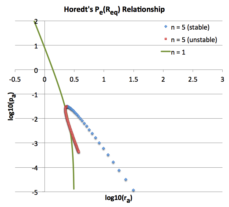
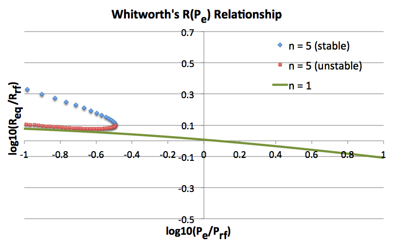
The solid green curve in the two top panels of Figure 1 shows how <math>R_\mathrm{eq}</math> varies with the applied external pressure <math>P_e</math> for this pressure-bounded <math>~n=1</math> model sequence. In the top-right panel, following the lead of Whitworth (1981, MNRAS, 195, 967) — for clarification, read the accompanying ASIDE — these two quantities have been respectively normalized (or, "referenced") to,

<math> R_\mathrm{rf}\biggr|_\mathrm{n=1} \equiv \biggl( \frac{3^2 \cdot 5}{2^4 \pi} \biggr)^{1/2} \biggl(\frac{K}{G}\biggr)^{1/2} ~~~\Rightarrow ~~~ \frac{R_\mathrm{eq}}{R_\mathrm{rf}} = \biggl( \frac{2^3}{3^2 \cdot 5} \biggr)^{1/2} \xi_e \, ; </math>

and,

<math> P_\mathrm{rf}\biggr|_\mathrm{n=1} \equiv \frac{2^6 \pi}{3^4 \cdot 5^3} \biggl(\frac{G^3 M^2}{K^2}\biggr) ~~~\Rightarrow ~~~ \frac{P_e}{P_\mathrm{rf}} = \biggl( \frac{3^4 \cdot 5^3}{2^7} \biggr) \biggl[ \frac{\sin\xi_e}{\xi_e(\sin\xi_e - \xi_e \cos\xi_e )} \biggr]^2 \, . </math>

Note that this pair of mathematical expressions has been recorded to the immediate right of Whitworth's name in our <math>~n=1</math> summary table. In the top-left panel of Figure 1, the solid green curve shows the identical sequence, but plotted as <math>~\log(p_a)</math> versus <math>~log(r_a)</math>, for easier comparison with Horedt's work. The pair of mathematical expressions defining <math>~r_a(\xi_e)</math> and <math>~p_a(\xi_e)</math> has been recorded to the immediate right of Horedt's name in the same summary table.

Figure 1: Equilibrium R-P Diagram
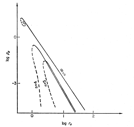
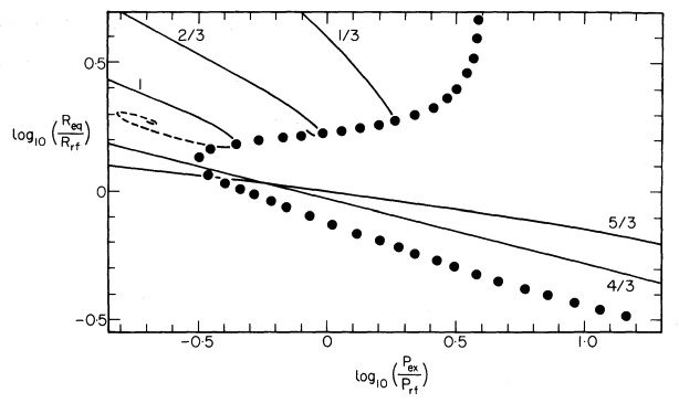
All of the plots shown in this figure illustrate how the equilibrium radius of a pressure-bounded polytrope varies with the applied external pressure. In the right-hand column, the log-log plots display a normalized <math>~P_e</math> along the horizontal axis and a normalized <math>~R_\mathrm{eq}</math> along the horizontal axis; in the left-hand column, these axes are flipped, and a different normalization is used. One primary intent of all the diagrams is to show that, for polytropic sequences having <math>~n > 3</math> (or, equivalently, sequences having <math>\gamma_g \equiv 1 + 1/n < 4/3),</math> no equilibrium models exist above some limiting external pressure.



Bottom Left [reproduction of Figure 1 from Horedt (1970)]: All three displayed sequences — <math>~n=4</math> (<math>~\gamma_g = 1.25</math>), <math>~n=5</math> (<math>~\gamma_g = 1.20</math>), and <math>~n=\infty</math> (<math>~\gamma_g = 1</math>, hence, isothermal) — exhibit an upper limit for the bounding pressure. Each sequence displays two segments — a solid segment and a dashed segment — indicating that, below the maximum allowed value of <math>~P_e</math>, it is possible to construct two (or more) equilibrium configurations; models lying along the solid segment of each displayed curve are expected to be dynamically stable while models lying along the dashed segments are unstable. Bottom Right [reproduction of Figure 1b from Whitworth (1981)]: Model sequences are shown for five different effective adiabatic indexes — <math>~\gamma_g = 1/3,~ 2/3,~ 1,~ 4/3,</math> and <math>~ 5/3</math> — corresponding, respectively, to polytropic indexes <math>~n = -2/3, -1/3, \infty, ~3/2, </math> and <math>~3</math>. The three sequences having <math>~\gamma_g < 4/3</math> exhibit an upper limit for the bounding pressure. Both the stable (solid) curve segment and the unstable (dashed) curve segment are drawn for the isothermal <math>~(\gamma_g = 1)</math> sequence, which is also displayed (as the <math>~n=\infty</math> sequence) in Horedt's diagram. Top: Plots that we have generated for direct comparison with Horedt's diagram (left) and with Whitworth's diagram (right). Both plots display only the two sequences that are analytically prescribable: <math>~n=1</math> (<math>~\gamma_g = 2</math>) and <math>~n=5</math> (<math>~\gamma_g = 1.20</math>). Along the <math>~n=1</math> (green) sequence, stable equilibrium models can be constructed for all values of <math>~P_e</math>. Along the <math>~n=5</math> sequence, equilibrium models only exist for values of <math>~P_e</math> less than the critical value, <math>~P_\mathrm{max} = (2^5\cdot 3^9/5^9) P_\mathrm{rf} = (3^{12}/2^{24}) P_\mathrm{Horedt}</math>; below this critical pressure, the sequence has two branches denoted by blue diamonds (stable models) and red squares (unstable models).

Overlap with Stahler's Presentation

We can invert the above expression for <math>~P_e(K,M)</math> to obtain the following expression for <math>~M(K,P_e)</math>:

<math>~M= K \biggl[\frac{2}{\pi} \cdot \frac{P_e}{G^3} \biggr]^{1/2} \biggl[ \frac{\xi_e(\sin\xi_e - \xi_e \cos\xi_e )}{\sin\xi_e} \biggr]</math> .

If, following Stahler's lead, we normalize this expression by <math>~M_\mathrm{norm}</math> (evaluated for <math>~n=1</math>) and we normalize the above expression for <math>~R_\mathrm{eq}</math> by <math>~R_\mathrm{norm}</math> (evaluated for <math>~n=1</math>), we obtain,

<math> \frac{M}{M_\mathrm{norm}} </math>	<math>~=~</math>	<math> K \biggl[\frac{2}{\pi} \cdot \frac{P_e}{G^3} \biggr]^{1/2} \biggl[ \frac{\xi_e(\sin\xi_e - \xi_e \cos\xi_e )}{\sin\xi_e} \biggr] \biggl[ \biggl( \frac{G}{2} \biggr)^{3/2} K^{-1} P_\mathrm{ex}^{-1/2} \biggr] </math>
	<math>~=~</math>	<math> (4\pi)^{-1/2} \biggl[ \frac{\xi_e(\sin\xi_e - \xi_e \cos\xi_e )}{\sin\xi_e} \biggr] \, , </math>
<math> \frac{R_\mathrm{eq}}{R_\mathrm{norm}} </math>	<math>~=~</math>	<math> \biggl[ \frac{K}{2\pi G} \biggr]^{1/2} \xi_e \biggl[ \frac{G}{2K} \biggr]^{1/2} = (4\pi)^{-1/2} \xi_e \, . </math>

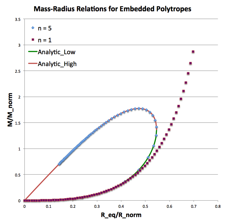
Figure 2: Equilibrium Mass-Radius Diagram
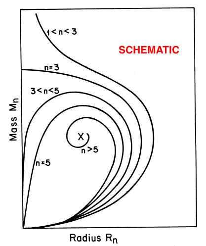
	Top: A slightly edited reproduction of Figure 17 in association with Appendix B of Stahler (1983, ApJ, 268, 165). Stahler's figure caption reads, in part, "Mass-radius relation for bounded polytropes (schematic). Each curve is labeled by the appropriate value or range" of <math>~n</math> … "As the cloud density increases from unity, all curves leave the origin with the same slope …" Bottom: Curves depict the exact, analytically derived mass-radius relationship for truncated <math>~n = 1</math> (purple squares) and <math>~n = 5</math> (blue diamonds) polytropes that are embedded in an external medium of pressure <math>~P_e</math>; the relevant mathematical expressions are presented to the immediate right of Stahler's name in, respectively, our <math>~n=1</math> summary table and our <math>~n=5</math> summary table. As the dimensionless truncation radius, <math>~\xi_e</math>, increases steadily from zero, both curves exhibit very similar behavior up to <math>~M_n \equiv M/M_\mathrm{norm} \approx 0.5</math>; thereafter the normalized mass and normalized radius continue to steadily increase along the <math>~n = 1</math> sequence, but the <math>~n = 5</math> sequence eventually bends back on itself, returning to the origin as <math>~\xi_e \rightarrow \infty</math>. Comparison: The monotonic <math>P-R</math> behavior of the analytically derived solution for <math>~n</math> = 1 <math>(\gamma_g = 2)</math>, shown above, is consistent with the behavior of the numerically derived solutions presented by Whitworth for slightly lower values of <math>\gamma_g</math> = 5/3 and 4/3. The analytically derived solution for <math>~n</math> = 5 <math>(\gamma_g = 6/5)</math> shows that, above some limiting pressure, no equilibrium configuration exists; this is consistent with the behavior of the numerically derived solutions presented by Whitworth for all values of <math>\gamma_g < 4/3 \, .</math>

Tabular Summary (n=1)

Properties of <math>~n=1</math> Polytropes Embedded in an External Medium of Pressure <math>~P_e</math>
(and, accordingly, truncated at radius <math>~\xi_e</math>)

<math> ~\theta_1 = \frac{\sin\xi_e}{\xi_e} </math>

and

<math> ~\frac{d\theta_1}{d\xi} \biggr|_{\xi_e} = \frac{\cos\xi_e}{\xi_e} - \frac{\sin\xi_e}{\xi_e^2} </math>

Horedt (1970)
for
fixed <math>~(M,K_n)</math>

<math> ~r_a = \frac{R_\mathrm{eq}}{R_\mathrm{Horedt}} = \xi_e </math>

<math> ~p_a = \frac{P_e}{P_\mathrm{Horedt}} = \biggl[ \frac{\sin\xi_e}{\xi_e(\sin\xi_e - \xi_e \cos\xi_e )} \biggr]^2 </math>

Whitworth (1981)
for
fixed <math>~(M,K_n)</math>

<math> \frac{R_\mathrm{eq}}{R_\mathrm{rf}} = \biggl( \frac{2^3}{3^2 \cdot 5} \biggr)^{1/2} \xi_e </math>

<math> \frac{P_e}{P_\mathrm{rf}} = \biggl( \frac{3^4 \cdot 5^3}{2^7} \biggr) \biggl[ \frac{\sin\xi_e}{\xi_e(\sin\xi_e - \xi_e \cos\xi_e )} \biggr]^2 </math>

Stahler (1983)
for
fixed <math>~(P_e,K_n)</math>

<math> \frac{R_\mathrm{eq}}{R_\mathrm{norm}} = (4\pi)^{-1/2} \xi_e </math>

<math> \frac{M}{M_\mathrm{norm}} = (4\pi)^{-1/2} \biggl[ \frac{\xi_e(\sin\xi_e - \xi_e \cos\xi_e )}{\sin\xi_e} \biggr] </math>

NOTE: None of the analytic expressions for the dimensionless radius, pressure, or mass presented in this table explicitly appear in the referenced articles by Horedt, by Whitworth, or by Stahler but, as is discussed fully above, they are straightforwardly derivable from the more general relations that appear in these papers.

<math>~n</math> = 5 Polytrope

Drawing from the earlier discussion of isolated polytropes, we will reference various radial locations within a spherical <math>~n</math> = 5 polytrope by the dimensionless radius,

<math> \xi \equiv \frac{r}{a_\mathrm{n=5}} , </math>

where,

<math> a_{n=5} = \biggr[ \frac{(n+1)K}{4\pi G} \rho_c^{(1/n - 1)} \biggr]^{1/2}_{n=5} = \biggr[ \frac{3K}{2\pi G} \biggr]^{1/2} \rho_c^{-2/5} \, . </math>

The solution to the Lane-Emden equation for <math>~n = 5</math> is,

<math> ~\theta_5 </math>

<math> \biggl(1+\frac{\xi^2}{3} \biggr)^{-1/2} \, , </math>

hence,

<math> \frac{d\theta_5}{d\xi} </math>

<math> - \frac{\xi}{3}\biggl(1+\frac{\xi^2}{3} \biggr)^{-3/2} \, . </math>