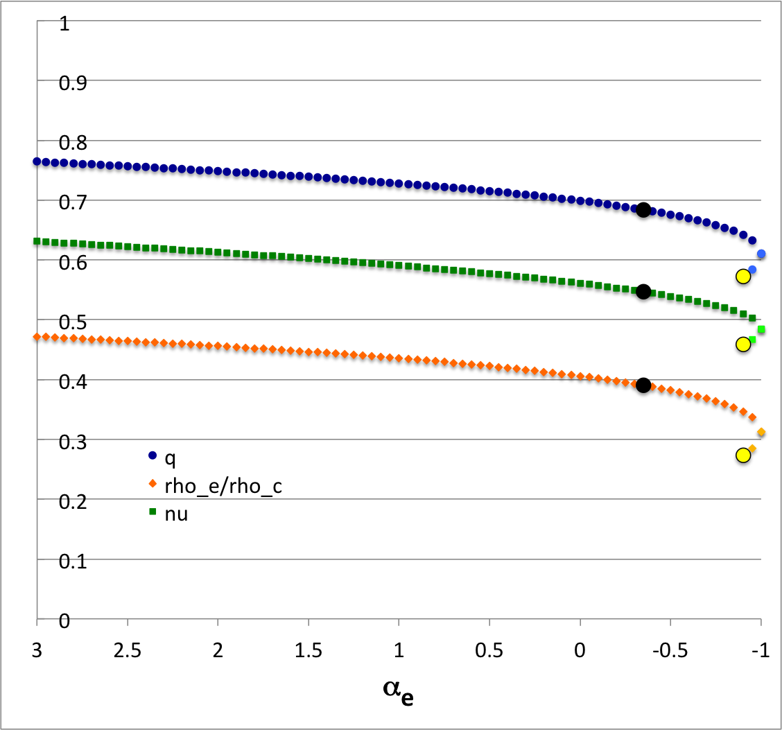
User:Tohline/Appendix/Ramblings/Additional Analytically Specified Eigenvectors for Zero-Zero Bipolytropes
Searching for Additional Eigenvectors of Zero-Zero Bipolytropes
This chapter is an extension of two accompanying discussions: The original discovery and detailed derivation; and the more readable, summary.

|
|---|
| | Tiled Menu | Tables of Content | Banner Video | Tohline Home Page | |
In our accompanying summary, we have demonstrated how analytically specified eigenvectors can be constructed for the mode labeled, <math>~(\ell, j) = (2,1)</math>. This was done by specifying <math>~\gamma_e</math>, then solving a quartic equation for <math>~q</math>. Shortly after completing this summary chapter, we noticed that an alternate approach may be to specify <math>~q</math>, then solve for <math>~\gamma_e</math>; and this path may be simpler because it may only involve solution of a quadratic equation. (Actually, we later have realized that the relevant equation is cubic, rather than quadratic. This is nevertheless simpler than the quartic equation.) If this proves to be the case, then it may also be possible to analytically construct eigenvectors of additional modes. Let's see.
|
CAUTION! All of the "core" eigenfunction expressions are suspect because (I think!) they have been developed herein under the assumption that <math>~g^{-2} = (1+2q^3)^2</math>, whereas the relation should read,
|
Seek Alternate Solution to Mode21 <math>~(\ell,j) = (2,1)</math>
Setup21
According to STEP 4 in our accompanying summary discussion, we need to solve the following "derivative matching" expression:
|
<math>~\frac{14(1+2\Chi)^2}{7(1+2\Chi)^2 - 5(1+8\Chi)}</math> |
<math>~=</math> |
<math>~ \frac{c_0 + (c_0 + 3)A_{21}\Chi + (c_0 + 6)A_{21}B_{21} \Chi^2}{1 + A_{21}\Chi + A_{21}B_{21}\Chi^2} </math> |
where, recognizing that, <math>~\alpha_e = c_0(c_0+2) \, ,</math>
|
<math>~A_{21}</math> |
<math>~\equiv</math> |
<math>~\biggl[ \frac{c_0(c_0+5) - (c_0 + 6)(c_0 + 11)}{(c_0 + 3)(c_0+5) - \alpha_e}\biggr] </math> |
|
|
<math>~=</math> |
<math>~\biggl[ \frac{c_0^2 + 5c_0 - (c_0^2 + 17c_0 + 66)}{(c_0^2 + 8c_0 + 15) - (c_0^2+2c_0)}\biggr] </math> |
|
|
<math>~=</math> |
<math>~-\biggl( \frac{ 4c_0 + 22}{2c_0 + 5}\biggr) \, ,</math> |
|
<math>~B_{21}</math> |
<math>~\equiv</math> |
<math>~\biggl[ \frac{(c_0+3)(c_0+8) - (c_0 + 6)(c_0 + 11)}{(c_0 + 6)(c_0+8) - \alpha_e}\biggr] </math> |
|
|
<math>~=</math> |
<math>~\biggl[ \frac{(c_0^2 +11c_0 + 24) - (c_0^2 + 17c_0 + 66)}{(c_0^2+14c_0+48) - (c_0^2 + 2c_0)}\biggr] </math> |
|
|
<math>~=</math> |
<math>~-\biggl( \frac{c_0 + 7 }{2c_0+8}\biggr) \, . </math> |
Here, we assume that <math>~\Chi \equiv q^3</math> is specified and seek the corresponding value of <math>~c_0</math>. Given that the LHS of this matching relation is known once <math>~\Chi</math> has been specified, in order to simplify notation we will also define,
|
<math>~Q</math> |
<math>~\equiv</math> |
<math>~\frac{14(1+2\Chi)^2}{7(1+2\Chi)^2 - 5(1+8\Chi )} \, .</math> |
Then the matching relation becomes,
|
<math>~Q</math> |
<math>~=</math> |
<math>~ \frac{c_0 + (c_0 + 3)A_{21}\Chi + (c_0 + 6)A_{21}B_{21} \Chi^2}{1 + A_{21}\Chi + A_{21}B_{21}\Chi^2} </math> |
|
<math>~\Rightarrow~~~ 0</math> |
<math>~=</math> |
<math>~[c_0 + (c_0 + 3)A_{21}\Chi + (c_0 + 6)A_{21}B_{21} \Chi^2 ] - Q[1 + A_{21}\Chi + A_{21}B_{21}\Chi^2 ] </math> |
|
|
<math>~=</math> |
<math>~\biggl[c_0 - (c_0 + 3)\biggl( \frac{ 4c_0 + 22}{2c_0 + 5}\biggr)\Chi + (c_0 + 6)\biggl( \frac{ 4c_0 + 22}{2c_0 + 5}\biggr)\biggl( \frac{c_0 + 7 }{2c_0+8}\biggr) \Chi^2 \biggr] - Q\biggl[1 - \biggl( \frac{ 4c_0 + 22}{2c_0 + 5}\biggr)\Chi + \biggl( \frac{ 4c_0 + 22}{2c_0 + 5}\biggr)\biggl( \frac{c_0 + 7 }{2c_0+8}\biggr)\Chi^2 \biggr] </math> |
|
|
<math>~=</math> |
<math>~\biggl[c_0(2c_0+5)(2c_0+8) - (c_0 + 3)(2c_0+8)( 4c_0 + 22)\Chi + (c_0 + 6)( 4c_0 + 22)(c_0 + 7 ) \Chi^2 \biggr] </math> |
|
|
|
<math>~ - Q\biggl[(2c_0+5)(2c_0+8) - (2c_0+8)( 4c_0 + 22)\Chi + ( 4c_0 + 22)( c_0 + 7 )\Chi^2 \biggr] </math> |
|
|
<math>~=</math> |
<math>~\biggl\{c_0(4c_0^2 + 26c_0 + 40) + ( 4c_0 + 22)\Chi [(c_0^2 + 13c_0 + 42 ) \Chi- (2c_0^2 +14c_0 +24)] \biggr\} </math> |
|
|
|
<math>~ - Q\biggl\{ (4c_0^2 + 26c_0 + 40) + ( 4c_0 + 22)\Chi [c_0(\Chi-2) + (7\Chi-8) ] \biggr\} </math> |
|
|
<math>~=</math> |
<math>~4c_0^3 +[ 26 - 4Q]c_0^2 + [40 - 26Q]c_0 - 40Q </math> |
|
|
|
<math>~ + ( 4c_0 + 22)\Chi \biggl\{ [\Chi - 2]c_0^2 + [13\Chi -14 -Q (\Chi-2) ]c_0 + [42\Chi -Q (7\Chi-8) -24] \biggr\} </math> |
|
|
<math>~=</math> |
<math>~4c_0^3 +[ 26 - 4Q]c_0^2 + [40 - 26Q]c_0 - 40Q </math> |
|
|
|
<math>~ + 4\Chi[\Chi - 2]c_0^3 + 4\Chi[13\Chi -14 -Q (\Chi-2) ]c_0^2 + 4\Chi[42\Chi -Q (7\Chi-8) -24]c_0 </math> |
|
|
|
<math>~ + 22\Chi[\Chi - 2]c_0^2 + 22\Chi[13\Chi -14 -Q (\Chi-2) ]c_0 + 22\Chi[42\Chi -Q (7\Chi-8) -24] \, . </math> |
Solve Cubic Equation
Here we draw from a separate discussion of solutions to a cubic equation.
|
Using <math>~y</math> in place of <math>~c_0</math>, this "derivative matching" relation can be written in the form of a standard cubic equation. Specifically,
where,
As is well known and documented — see, for example Wolfram MathWorld or Wikipedia's discussion of the topic — the roots of any cubic equation can be determined analytically. In order to evaluate the root(s) of our particular cubic equation, we have drawn from the utilitarian online summary provided by Eric Schechter at Vanderbilt University. For a cubic equation of the general form, <math>~ay^3 + by^2 + cy + d = 0 \, ,</math> a real root is given by the expression, <math>~ y = p + \{z + [z^2 + (r-p^2)^3]^{1/2}\}^{1/3} + \{z - [z^2 + (r-p^2)^3]^{1/2}\}^{1/3} \, ,</math> where, <math>~p \equiv -\frac{b}{3a} \, ,</math> <math>~z \equiv \biggl[p^3 + \frac{bc-3ad}{6a^2} \biggr] \, ,</math> and <math>~r=\frac{c}{3a} \, .</math> (There is also a pair of imaginary roots, but they are irrelevant in the context of our overarching astrophysical discussion.) |
Upon evaluation, we have found that the expression inside of the square root is negative over the region of parameter space that is of most physical interest. Hence, we need to call upon a separate discussion in which the cube root of complex numbers was discussed.
|
We'll shift to Wolfram's notation; specifically,
Then, after defining, <math>~D \equiv Q^3 + R^2 = z^2 + (r-p^2)^3 \, ;</math> <math>~S^3 \equiv R+ \sqrt{D} \, ;</math> and <math>~T^3 \equiv R- \sqrt{D} \, ;</math> Wolfram states that the three roots of the cubic equation are (the first one being identical to the "real" root identified above),
Now, whenever <math>~D</math> is intrinsically negative, we need to treat both <math>~S^3</math> and <math>~T^3</math> as complex numbers. If we define,
then we can write,
As is explained in this online resource, both <math>~S</math> and <math>~T</math> must formally submit to three separate roots tagged by the integer index, <math>~(j=0,1,2)</math>. Working only with the <math>~j=0</math> root for both, we find that the above expressions for the three roots of our cubic equation become,
|
We have deduced empirically that <math>~y_3</math> is the root that is physically relevant in our case. That is to say, for a given <math>~0 < q < 1</math>,
<math>~c_0 = p - \mathfrak{r}^{1 / 3} \biggl[ \cos\biggl(\frac{\theta}{3}\biggr) - \sqrt{3} \sin\biggl(\frac{\theta}{3}\biggr) \biggr] \, .</math>
In turn, for a given value of <math>~q</math>, the corresponding value of <math>~\alpha_e</math> is obtained via the relation, <math>~\alpha_e = c_0(c_0 + 2)</math>.
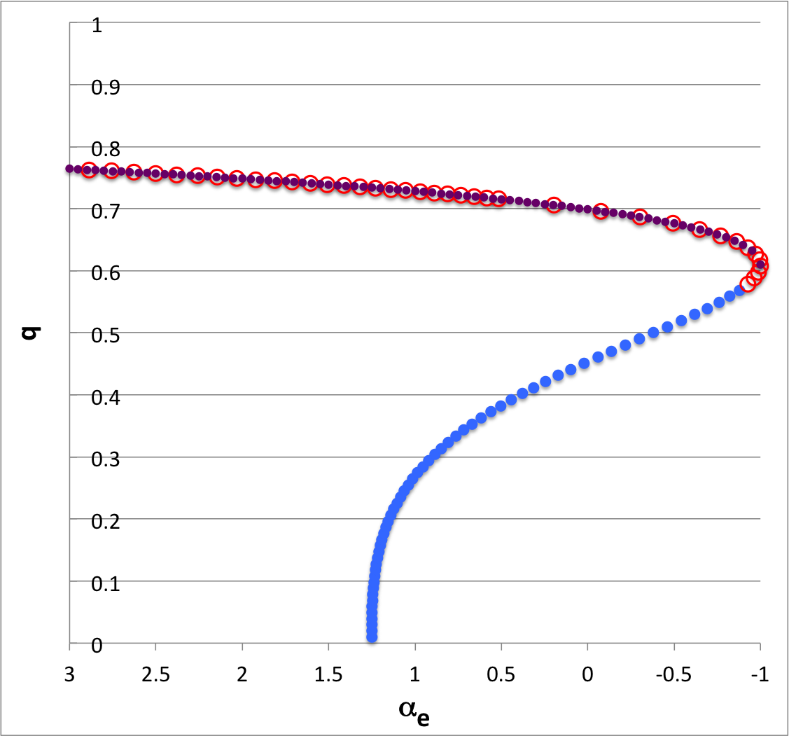
The right-hand panel of Figure 1 presents a plot of this <math>~c_0(q)</math> function; actually what has been plotted is the inverted relation, <math>~q(\alpha_e)</math>. The open, red circular markers trace the portion of the function that provides physically viable solutions, in the sense that the corresponding value of <math>~\alpha_c</math> lies between the values, negative one and three; the filled, light=blue circular markers identify roots of the cubic equation that are not physically viable.
In the left-hand panel of Figure 1, we re-display a plot that has been discussed in an accompanying chapter. It contains a plot (blue markers) of the same same <math>~q(\alpha_e)</math> function but, this time, as determined from the root of a quartic equation. In order to illustrate more clearly that the two curves are the same, we have plotted the quartic solution (small, purple circular markers) on top of the cubic solution in the right-hand panel.
Illustration21
|
Analytically Definable Eigenvectors in <math>~(n_c, n_e) = (0,0)</math> Bipolytropes Quantum Numbers: <math>~(\ell,j) = (2,1)</math> |
|
|---|---|
| Analyzable Model Sequence | One Example Eigenfunction |
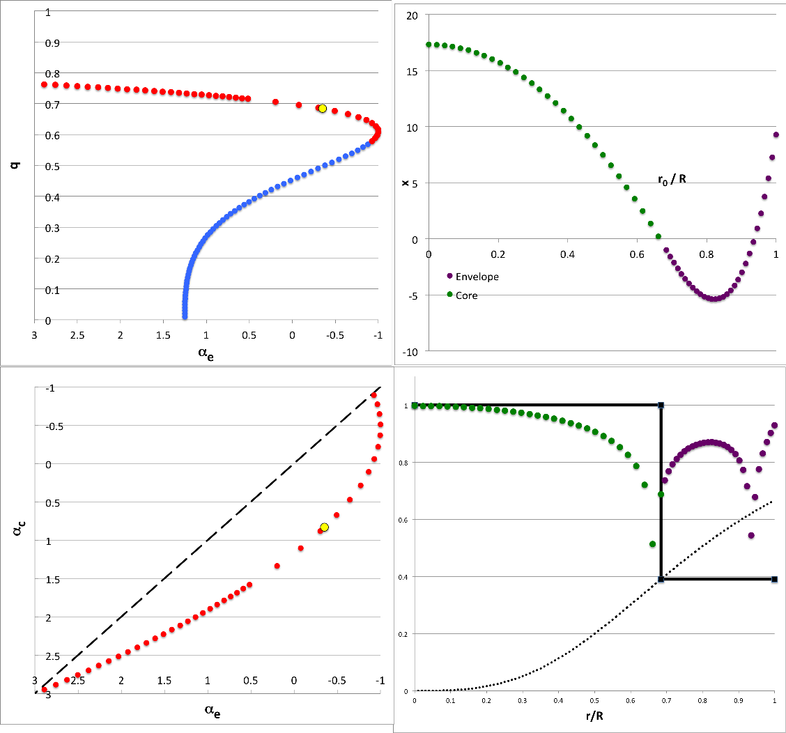
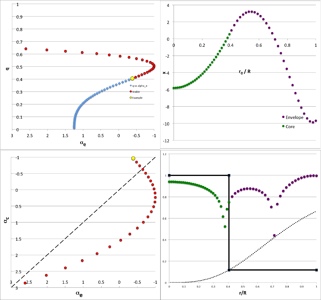
Top-Left Panel: Plotted points show how the location of the core/envelope interface, <math>~q \equiv r_i/R</math>, varies with <math>~\alpha_e \equiv (3-4/\gamma_e)</math> — where <math>~\gamma_e</math> is the adiabatic exponent of the envelope — in equilibrium models that are amenable to analytic modal analysis for quantum numbers, <math>~(\ell,j) = (2,1)</math>. Red (alternatively, blue) markers identify models for which the corresponding value of the adiabatic exponent of the core [see bottom-left panel] falls inside (alternatively, outside) the physically viable range, namely, <math>~1 \le \gamma_c \le \infty</math>. The yellow circular marker identifies the model whose analytically determined eigenfunction is displayed on the right, as an example.
Bottom-Left Panel: Plotted points show how <math>~\alpha_c \equiv (3-4/\gamma_c)</math> varies with <math>~\alpha_e</math> over the physically viable parameter range, <math>~-1 \le \alpha \le 3</math>. Both axes have been flipped so that incompressible models <math>~(\gamma = \infty)</math> lie on the left/bottom while isothermal models <math>~(\gamma =1)</math> lie on the right/top. The core is more compressible than the envelope in models that lie above and to the left of the black-dashed, diagonal line. The yellow circular marker identifies the same example model as it does in the top-left panel.
Top-Right Panel: Displays — as a function of the fractional radius, <math>~r_0/R = q\xi</math> — the analytically determined eigenfunction for the <math>~(\ell,j) = (2,1)</math> mode in the model identified by the yellow circular marker in both left-hand panels, for which,
<math>~\alpha_e =-0.35</math> <math>~\Rightarrow</math> <math>~c_0~\mathrm{(plus)} = -0.1937742</math>
and, correspondingly (via our separate solution of the governing quartic equation), <math>~(q,\alpha_c) = (0.6840119, +0.8326585)</math>. (This same plot appears in Figure 1 of our accompanying summary.) Specifically, over the radial interval, <math>~0 \le \xi \le 1</math>, the green markers trace the core's contribution to the combined eigenfunction, namely,
|
<math>~x_{j=1} |_\mathrm{core}</math> |
<math>~=</math> |
<math>~ \frac{5 (1+8q^3) - 7 (1+2q^3)^2 \xi^2}{5 (1+8q^3)-7(1+2q^3)^2} \, ;</math> |
and, over the radial interval, <math>~1 \le \xi \le 1/q</math>, the purple markers trace the envelope's contribution to the combined eigenfunction, namely,
|
<math>~x_{\ell=2} |_\mathrm{env}</math> |
<math>~=</math> |
<math>~ \xi^{c_0}\biggl[ \frac{ 1 + q^3 A_{21} \xi^{3} + q^6 A_{21}B_{21}\xi^{6} }{ 1 + q^3 A_{21} + q^6 A_{21}B_{21} }\biggr] \, , </math> |
where the coefficients, <math>~A_{21}, B_{21}</math>, are as defined above in terms of the parameter, <math>~c_0</math>. The corresponding eigenfrequency is, from the perspective of the core,
|
<math>~\frac{3\omega^2}{2\pi G \rho_c}</math> |
<math>~=</math> |
<math>~20\gamma_c - 8 = \frac{8(7 + \alpha_c)}{3-\alpha_c} \approx 28.9115809\, ;</math> |
and, from the perspective of the envelope,
|
<math>~\frac{3\omega^2}{2\pi G \rho_c}</math> |
<math>~=</math> |
<math>~3\gamma_e\biggl[\alpha_e + 5c_0 + 22\biggr] \frac{\rho_e}{\rho_c} \approx 28.9115807\, ,</math> |
where the relevant density ratio is, <math>~\rho_e/\rho_c = 2q^3/(1+2q^3) \approx 0.3902664</math>.
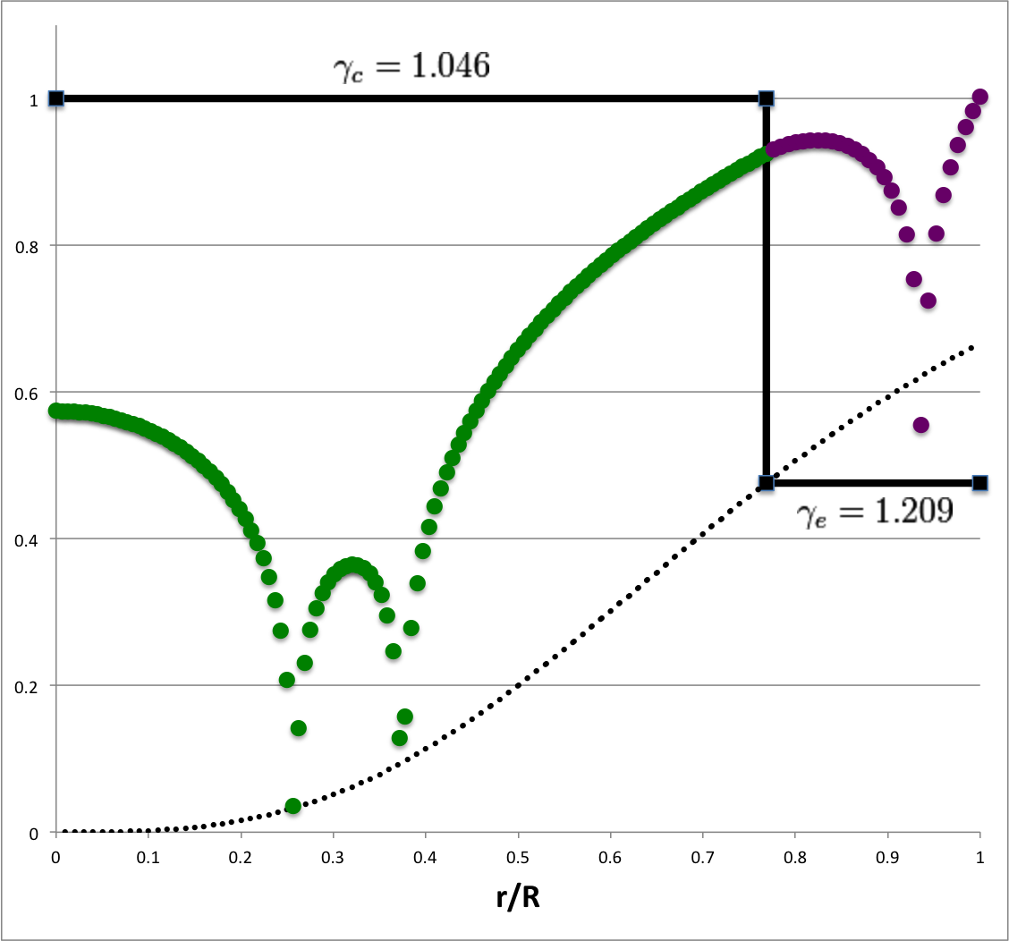
Bottom-Right Panel: The green and purple markers present the same eigenfunction-amplitude information, <math>~x(r/R)</math>, as in the Top-Right panel, but on a logarithmic scale. Specifically, in this plot, the vertical displacement of the green and purple markers is given by the expression,
|
<math>~y</math> |
<math>~=</math> |
<math>~\tfrac{1}{8} \log_{10}[x^2 + \epsilon^2] + y_\mathrm{shift} \, ,</math> |
where, for plotting purposes, we have used, <math>~\epsilon = 10^{-5}</math>, and have set <math>~y_\mathrm{shift}</math> to a value that ensures that <math>~y \approx 1</math> at the outer edge. In this type of log-amplitude plot, the eigenfunction's various nodes — that is, radial locations where <math>~x</math> passes through zero — are highlighted; here, specifically, there is one node inside the core and one node resides in the envelope. Using the vertical coordinate to represent, instead, the configuration's mass-density normalized to its central value, <math>~\rho/\rho_c</math>, the solid black line segments trace the unperturbed density distribution throughout this specific <math>~(n_c, n_e) = (0,0)</math> bipolytrope. Throughout the core, <math>~\rho/\rho_c = 1</math>; then, at the location of the interface <math>~(r_i/R = q \approx 0.684)</math>, the density abruptly drops to its envelope value <math>~(\rho/\rho_c = \rho_e/\rho_c \approx 0.39)</math>.
NOTE: As may be ascertained from our general discussion of the structural properties of <math>~(n_c, n_e) = (0,0)</math> bipolytropes, equilibrium "zero-zero" bipolytropes can be constructed with the envelope/core interface parameter set to any value across the range, <math>~0 \le q \le 1</math>; and for any chosen value of <math>~q</math>, the envelope/core density ratio can, in principle, be set to any value, <math>~0 \le \rho_e/\rho_c \le 1</math>. We have not, however, been able to analytically solve the relevant pair of linear-adiabatic wave equations (LAWEs) for this entire set of equilibrium models. Instead, our ability to derive analytically prescribed eigenvectors is limited by the constraint,
|
<math>~\frac{\rho_e}{\rho_c}</math> |
<math>~=</math> |
<math>~\frac{2q^3}{1+2q^3} = \frac{2(r_i/R)^3}{1+2(r_i/R)^3}\, .</math> |
The black-dotted curve in the Bottom-Right Panel displays the behavior of this constraint; accordingly, the step function depicted by the solid black line segments must necessarily drop from unity to a point on this black-dotted curve for any equilibrium model — such as the example illustrated here — that has an analytically prescribable radial-oscillation eigenvector.
Try Mode22 <math>~(\ell,j) = (2,2)</math>
Setup22
In this case we need to replace the core eigenfunction segment that was specified in STEP 3 in our separate discussion of mode <math>~(\ell,j) = (2,1)</math> with the following:
|
<math>~x_{j=2} |_\mathrm{core}</math> |
<math>~=</math> |
<math>~ \frac{35(1+8q^3)^2 - 126 (1+8q^3) (1+2q^3)^2 \xi^2 + 99 (1+2q^3)^4 \xi^4 }{35(1+8q^3)^2 - 126(1+8q^3) (1+2q^3)^2 + 99 (1+2q^3)^4 } </math> |
So, following the procedure outlined in STEP 4 of our separate discussion, the requirement that the first derivatives match at the interface becomes,
|
<math>~\frac{ - 252 (1+8q^3) (1+2q^3)^2 + 396 (1+2q^3)^4 }{35(1+8q^3)^2 - 126(1+8q^3) (1+2q^3)^2 + 99 (1+2q^3)^4 }</math> |
<math>~=</math> |
<math>~ \frac{c_0 + (c_0 + 3)A_{22}q^3 + (c_0 + 6)A_{22}B_{22} q^6}{1 + A_{22}q^3 + A_{22}B_{22}q^6} \, , </math> |
where,
|
<math>~A_{22}</math> |
<math>~=</math> |
<math>~A_{21} = -\biggl( \frac{ 4c_0 + 22}{2c_0 + 5}\biggr) \, ,</math> |
|
<math>~B_{22}</math> |
<math>~=</math> |
<math>~B_{21} = -\biggl( \frac{c_0 + 7 }{2c_0+8}\biggr) \, . </math> |
So, as described above, in order to determine <math>~c_0</math> for any specified value of <math>~q</math> — or, equivalently, <math>~\Chi \equiv q^3</math> — we simply need to replace <math>~Q_{21}</math> with <math>~Q_{22}</math> in the definition of the coefficient of each term in the cubic expression, where,
|
<math>~Q_{22}</math> |
<math>~\equiv</math> |
<math>~ \frac{ - 252 (1+8q^3) (1+2q^3)^2 + 396 (1+2q^3)^4 }{35(1+8q^3)^2 - 126(1+8q^3) (1+2q^3)^2 + 99 (1+2q^3)^4 }\, . </math> |
Finally, as explained in our summary discussion, in order for the two (dimensional) eigenfrequencies to match, the adiabatic exponent for the core must be,
|
<math>~ \gamma_c </math> |
<math>~=</math> |
<math>~\frac{1}{[ 6 + 2j(2j+5)] } \biggl\{ 8 + \gamma_e \biggl[2\alpha_e + (c_0 + 3\ell)(c_0 + 3\ell +5) \biggr]\frac{\rho_e}{\rho_c} \biggr\} \, . </math> |
Illustration22
|
Analytically Definable Eigenvectors in <math>~(n_c, n_e) = (0,0)</math> Bipolytropes Quantum Numbers: <math>~(\ell,j) = (2,2)</math> |
|
|---|---|
| Analyzable Model Sequence | One Example Eigenfunction |
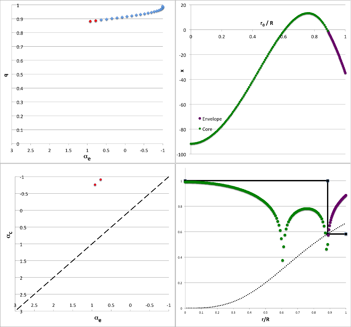
Top-Left Panel: Plotted points show how the location of the core/envelope interface, <math>~q \equiv r_i/R</math>, varies with <math>~\alpha_e \equiv (3-4/\gamma_e)</math> — where <math>~\gamma_e</math> is the adiabatic exponent of the envelope — in equilibrium models that are amenable to analytic modal analysis for quantum numbers, <math>~(\ell,j) = (2,2)</math>. Red (alternatively, blue) markers identify models for which the corresponding value of the adiabatic exponent of the core [see bottom-left panel] falls inside (alternatively, outside) the physically viable range, namely, <math>~1 \le \gamma_c \le \infty</math>. The red marker that is farthest to the left identifies the model whose analytically determined eigenfunction is displayed, as an example, in the right-hand panels.
Bottom-Left Panel: Plotted points (only 2, here!) show how <math>~\alpha_c \equiv (3-4/\gamma_c)</math> varies with <math>~\alpha_e</math> over the physically viable parameter range, <math>~-1 \le \alpha \le 3</math>. Both axes have been flipped so that incompressible models <math>~(\gamma = \infty)</math> lie on the left/bottom while isothermal models <math>~(\gamma =1)</math> lie on the right/top. The core is more compressible than the envelope in models that lie above and to the left of the black-dashed, diagonal line.
Top-Right Panel: Displays — as a function of the fractional radius, <math>~r_0/R = q\xi</math> — the analytically determined eigenfunction for the <math>~(\ell,j) = (2,2)</math> mode in the model identified by the red circular marker that is farthest to the left in both left-hand panels, for which,
<math>~q = \biggl[0.005 + 179\biggl( \frac{0.985}{200} \biggr) \biggr] = 0.886575</math>
and, correspondingly, <math>~(c_0, \alpha_e,\alpha_c) = (-2.332785, +0.7763158, -0.9146699)</math>. Specifically, over the radial interval, <math>~0 \le \xi \le 1</math>, the green markers trace the core's contribution to the combined eigenfunction, namely,
|
<math>~x_{j=2} |_\mathrm{core}</math> |
<math>~=</math> |
<math>~ \frac{35(1+8q^3)^2 - 126(1+8q^3) (1+2q^3)^2 \xi^2 + 99 (1+2q^3)^4 \xi^4 }{35(1+8q^3)^2 - 126(1+8q^3) (1+2q^3)^2 + 99 (1+2q^3)^4 } \, ;</math> |
and, over the radial interval, <math>~1 \le \xi \le 1/q</math>, the purple markers trace the envelope's contribution to the combined eigenfunction, namely,
|
<math>~x_{\ell=2} |_\mathrm{env}</math> |
<math>~=</math> |
<math>~ \xi^{c_0}\biggl[ \frac{ 1 + q^3 A_{22} \xi^{3} + q^6 A_{22}B_{22}\xi^{6} }{ 1 + q^3 A_{22} + q^6 A_{22}B_{22} }\biggr] \, , </math> |
where the coefficients, <math>~A_{22}, B_{22}</math>, are as defined above in terms of the parameter, <math>~c_0</math>. The corresponding eigenfrequency is, from the perspective of the core,
|
<math>~\frac{3\omega^2}{2\pi G \rho_c}</math> |
<math>~=</math> |
<math>~42\gamma_c - 8 = \frac{8(18 + \alpha_c)}{3-\alpha_c} \approx 34.915496 \, ;</math> |
and, from the perspective of the envelope,
|
<math>~\frac{3\omega^2}{2\pi G \rho_c}</math> |
<math>~=</math> |
<math>~3\gamma_e\biggl[\alpha_e + 5c_0 + 22\biggr] \frac{\rho_e}{\rho_c} \approx 34.915496 \, ,</math> |
where the relevant density ratio is, <math>~\rho_e/\rho_c = 2q^3/(1+2q^3) \approx 0.5822407</math>.
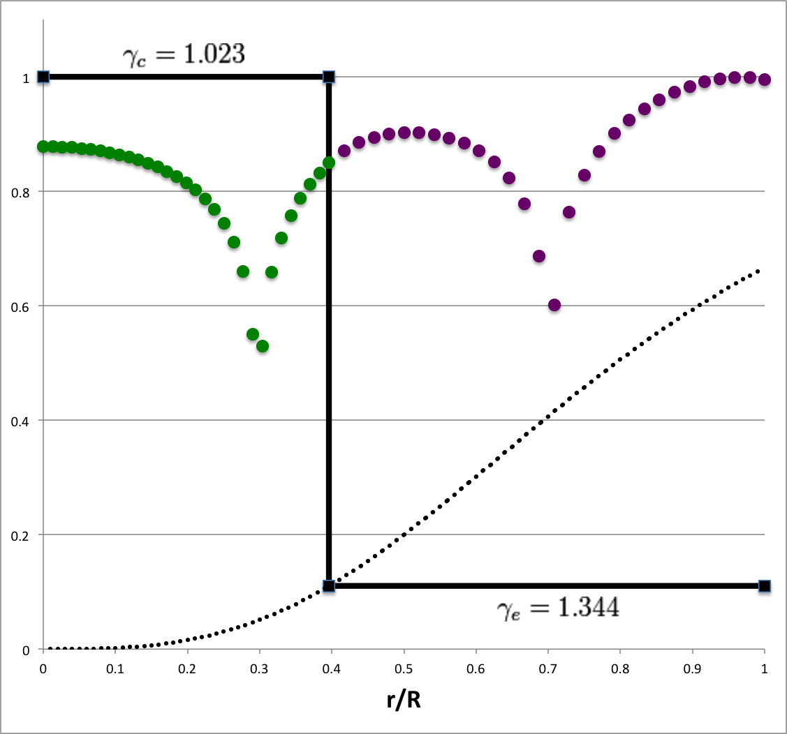
Bottom-Right Panel: The green and purple markers present the same eigenfunction-amplitude information, <math>~x(r/R)</math>, as in the Top-Right panel, but on a logarithmic scale. Specifically, in this plot, the vertical displacement of the green and purple markers is given by the expression,
|
<math>~y</math> |
<math>~=</math> |
<math>~\tfrac{1}{8} \log_{10}[x^2 + \epsilon^2] + y_\mathrm{shift} \, ,</math> |
where, for plotting purposes, we have used, <math>~\epsilon = 10^{-5}</math>, and have set <math>~y_\mathrm{shift}</math> to a value that ensures that <math>~y \approx 1</math> at the center of the configuration. In this type of log-amplitude plot, the eigenfunction's various nodes — that is, radial locations where <math>~x</math> passes through zero — are highlighted; here, specifically, there are two nodes inside the core and none in the envelope, although one of the nodes in the core lies just inside the core/envelope interface. Using the vertical coordinate to represent, instead, the configuration's mass-density normalized to its central value, <math>~\rho/\rho_c</math>, the solid black line segments trace the unperturbed density distribution throughout this specific <math>~(n_c, n_e) = (0,0)</math> bipolytrope. Throughout the core, <math>~\rho/\rho_c = 1</math>; then, at the location of the interface <math>~(r_i/R = q \approx 0.89)</math>, the density abruptly drops to its envelope value <math>~(\rho/\rho_c = \rho_e/\rho_c \approx 0.58)</math>.
NOTE: As may be ascertained from our general discussion of the structural properties of <math>~(n_c, n_e) = (0,0)</math> bipolytropes, equilibrium "zero-zero" bipolytropes can be constructed with the envelope/core interface parameter set to any value across the range, <math>~0 \le q \le 1</math>; and for any chosen value of <math>~q</math>, the envelope/core density ratio can, in principle, be set to any value, <math>~0 \le \rho_e/\rho_c \le 1</math>. We have not, however, been able to analytically solve the relevant pair of linear-adiabatic wave equations (LAWEs) for this entire set of equilibrium models. Instead, our ability to derive analytically prescribed eigenvectors is limited by the constraint,
|
<math>~\frac{\rho_e}{\rho_c}</math> |
<math>~=</math> |
<math>~\frac{2q^3}{1+2q^3} = \frac{2(r_i/R)^3}{1+2(r_i/R)^3}\, .</math> |
The black-dotted curve in the Bottom-Right Panel displays the behavior of this constraint; accordingly, the step function depicted by the solid black line segments must necessarily drop from unity to a point on this black-dotted curve for any equilibrium model — such as the example illustrated here — that has an analytically prescribable radial-oscillation eigenvector.
Try Mode31 <math>~(\ell,j) = (3,1)</math>
Setup31
In this case we need to replace the envelope eigenfunction segment that was specified in STEP 2 in our separate discussion of mode <math>~(\ell,j) = (2,1)</math> with the following: For the case of <math>~\ell=2</math>, this means that, throughout the envelope, the eigenfunction is,
|
<math>~x_{\ell=3} |_\mathrm{env}</math> |
<math>~=</math> |
<math>~ \xi^{c_0}\biggl[ \frac{ 1 + q^3 A_{31} \xi^{3} + q^6 A_{31}B_{31}\xi^{6} + q^9 A_{31}B_{31}C_{31}\xi^{9} }{ 1 + q^3 A_{31} + q^6 A_{31}B_{31} + q^9 A_{31}B_{31}C_{31} }\biggr] \, , </math> |
where, the values of the newly introduced coefficients,
|
<math>~A_{31}</math> |
<math>~\equiv</math> |
<math>~\biggl[ \frac{c_0(c_0+5) - (c_0 + 9)(c_0 + 14)}{(c_0 + 3)(c_0+5) - \alpha_e}\biggr] </math> |
|
|
<math>~=</math> |
<math>~\biggl[ \frac{c_0^2 + 5c_0 - (c_0^2 + 23c_0 + 126)}{(c_0^2 + 8c_0 + 15) - (c_0^2 + 2c_0)}\biggr] </math> |
|
|
<math>~=</math> |
<math>~\frac{- 6(c_0 + 7)}{2c_0 + 5 } \, ,</math> |
|
<math>~B_{31}</math> |
<math>~\equiv</math> |
<math>~\biggl[ \frac{(c_0+3)(c_0+8) - (c_0 + 9)(c_0 + 14)}{(c_0 + 6)(c_0+8) - \alpha_e}\biggr] </math> |
|
|
<math>~=</math> |
<math>~\biggl[ \frac{(c_0^2 + 11c_0 + 24) - (c_0^2 + 23c_0 + 126)}{(c_0^2 + 14c_0 +48) - (c_0^2 + 2c_0) }\biggr] </math> |
|
|
<math>~=</math> |
<math>~\frac{ - (6c_0 + 51)}{ 6(c_0 +4) } \, ,</math> |
|
<math>~C_{31}</math> |
<math>~\equiv</math> |
<math>~\biggl[ \frac{(c_0+6)(c_0+11) - (c_0 + 9)(c_0 + 14)}{(c_0 + 9)(c_0+11) - \alpha_e}\biggr] </math> |
|
|
<math>~=</math> |
<math>~\biggl[ \frac{(c_0^2 +17c_0 + 66) - (c_0^2 + 23 c_0 + 126)}{(c_0^2 + 20 c_0 + 99) - (c_0^2 + 2c_0) }\biggr] </math> |
|
|
<math>~=</math> |
<math>~\frac{- 2( c_0 + 10)}{3(2 c_0 + 11) } \, .</math> |
Then, after defining,
|
<math>~Q_{31}</math> |
<math>~\equiv</math> |
<math>~\frac{14(1+2\Chi)^2}{7(1+2\Chi)^2 - 5(1+8\Chi)} \, ,</math> |
the matching relation becomes,
|
<math>~Q_{31}</math> |
<math>~=</math> |
<math>~ \frac{c_0 + (c_0 + 3)A_{31}\Chi + (c_0 + 6)A_{31}B_{31} \Chi^2 + (c_0 + 9)A_{31}B_{31} C_{31}\Chi^3 }{1 + A_{31}\Chi + A_{31}B_{31}\Chi^2 + A_{31}B_{31}C_{31}\Chi^3 } </math> |
|
<math>~\Rightarrow~~~ 0</math> |
<math>~=</math> |
<math>~ [c_0 + (c_0 + 3)A_{31}\Chi + (c_0 + 6)A_{31}B_{31} \Chi^2 + (c_0 + 9)A_{31}B_{31} C_{31}\Chi^3 ] - Q_{31}[1 + A_{31}\Chi + A_{31}B_{31}\Chi^2 + A_{31}B_{31}C_{31}\Chi^3 ] </math> |
|
|
<math>~=</math> |
<math>~ \biggl[c_0 - (c_0 + 3)\cdot \frac{6(c_0 + 7)}{2c_0 + 5 } \cdot \Chi + (c_0 + 6) \cdot \frac{ 6(c_0 + 7)}{2c_0 + 5 } \cdot \frac{ (6c_0 + 51)}{ 6(c_0 +4) } \cdot \Chi^2 - (c_0 + 9)\cdot \frac{ 6(c_0 + 7)}{2c_0 + 5 } \cdot \frac{ (6c_0 + 51)}{ 6(c_0 +4) } \cdot \frac{ 2( c_0 + 10)}{3( 2c_0 + 11) } \cdot\Chi^3 \biggr] </math> |
|
|
|
<math>~ - Q_{31} \biggl[1 - \frac{ 6(c_0 + 7)}{2c_0 + 5 } \cdot \Chi + \frac{ 6(c_0 + 7)}{2c_0 + 5 } \cdot \frac{ (6c_0 + 51)}{ 6(c_0 +4) } \cdot \Chi^2 - \frac{ 6(c_0 + 7)}{2c_0 + 5 } \cdot \frac{ (6c_0 + 51)}{ 6(c_0 +4) } \cdot \frac{ 2( c_0 + 10)}{3( 2c_0 + 11) } \cdot \Chi^3 \biggr] </math> |
|
|
<math>~=</math> |
<math>~ \biggl[3c_0(2c_0 + 5)(c_0 +4)( 2c_0 + 11) - (c_0 + 3)(c_0 +4)3( 2c_0 + 11)\cdot 6(c_0 + 7) \cdot \Chi + (c_0 + 6) 3( 2c_0 + 11)\cdot (c_0 + 7) \cdot (6c_0 + 51) \cdot \Chi^2 - (c_0 + 9)\cdot (c_0 + 7) \cdot (6c_0 + 51)\cdot 2( c_0 + 10) \cdot\Chi^3 \biggr] </math> |
|
|
|
<math>~ - Q_{31} \biggl[ 3(2c_0 + 5)(c_0 +4)( 2c_0 + 11) - 18(c_0 + 7)(c_0 +4)( 2c_0 + 11) \cdot \Chi + 3( 2c_0 + 11)(c_0 + 7) \cdot (6c_0 + 51) \cdot \Chi^2 - 2(c_0 + 7) \cdot (6c_0 + 51) ( c_0 + 10) \cdot \Chi^3 \biggr] </math> |
Material that appears after this point in our presentation is under development and therefore
may contain incorrect mathematical equations and/or physical misinterpretations.
| Go Home |
Root of Quartic Equation
To solve this equation analytically, we follow the Summary of Ferrari's method that is presented in Wikipedia's discussion of the Quartic Function to identify the roots of an arbitrary quartic equation.
|
First, we adopt the shorthand notation:
where, in our particular case,
|
|
Now, define,
Then the four roots of the quartic equation are,
It is this fourth root that interests us, here. |
|
We have determined empirically that, in our specific case, the quantity,
is negative over the range of physically interesting values of <math>~\Chi</math>. Hence, the quantity, <math>~\Kappa^3</math>, is necessarily complex. Let's work carefully through a determination of <math>~\Kappa</math> and, by consequence, <math>~S</math>, in this situation.
where, <math>\Gamma \equiv \biggl[ \frac{\Delta_1^2}{4\Delta_0^3}\biggr]^{1/2} \, .</math> We therefore can state that, in the complex plane, the three roots <math>~(j=0,1,3)</math> of this expression are,
where, <math>\theta_\Kappa \equiv \cos^{-1}\Gamma \, .</math> Focusing on the simplest <math>~(j=0)</math> root, we have,
Because this expression does not contain an imaginary component, we understand that <math>~S</math> is real. |
Finally, as explained in our summary discussion, in order for the two (dimensional) eigenfrequencies to match, the adiabatic exponent for the core must be,
|
<math>~ \gamma_c </math> |
<math>~=</math> |
<math>~\frac{1}{ 6 + 2j(2j+5)] } \biggl\{ 8 + \gamma_e \biggl[2\alpha_e + (c_0 + 3\ell)(c_0 + 3\ell +5) \biggr]\frac{\rho_e}{\rho_c} \biggr\} </math> |
|
|
<math>~=</math> |
<math>~\frac{1}{ 20} \biggl\{ 8 + \gamma_e \biggl[2\alpha_e + (c_0 + 9)(c_0 + 14) \biggr]\frac{\rho_e}{\rho_c} \biggr\} \, , </math> |
where, the last expression follows from plugging in the desired mode's quantum numbers, <math>~(\ell,j) = (3,1)</math>, and, again, using the relation,
|
<math>~\Chi = q^3</math> |
<math>~=</math> |
<math>~\frac{\rho_e/\rho_c}{2(1-\rho_e/\rho_c)}</math> |
|
<math>~\Rightarrow ~~~ \frac{\rho_e}{\rho_c}</math> |
<math>~=</math> |
<math>~\frac{2\Chi}{1+2\Chi} \, .</math> |
Illustration31
|
Analytically Definable Eigenvectors in <math>~(n_c, n_e) = (0,0)</math> Bipolytropes Quantum Numbers: <math>~(\ell,j) = (3,1)</math> |
|
|---|---|
| Analyzable Model Sequence | One Example Eigenfunction |
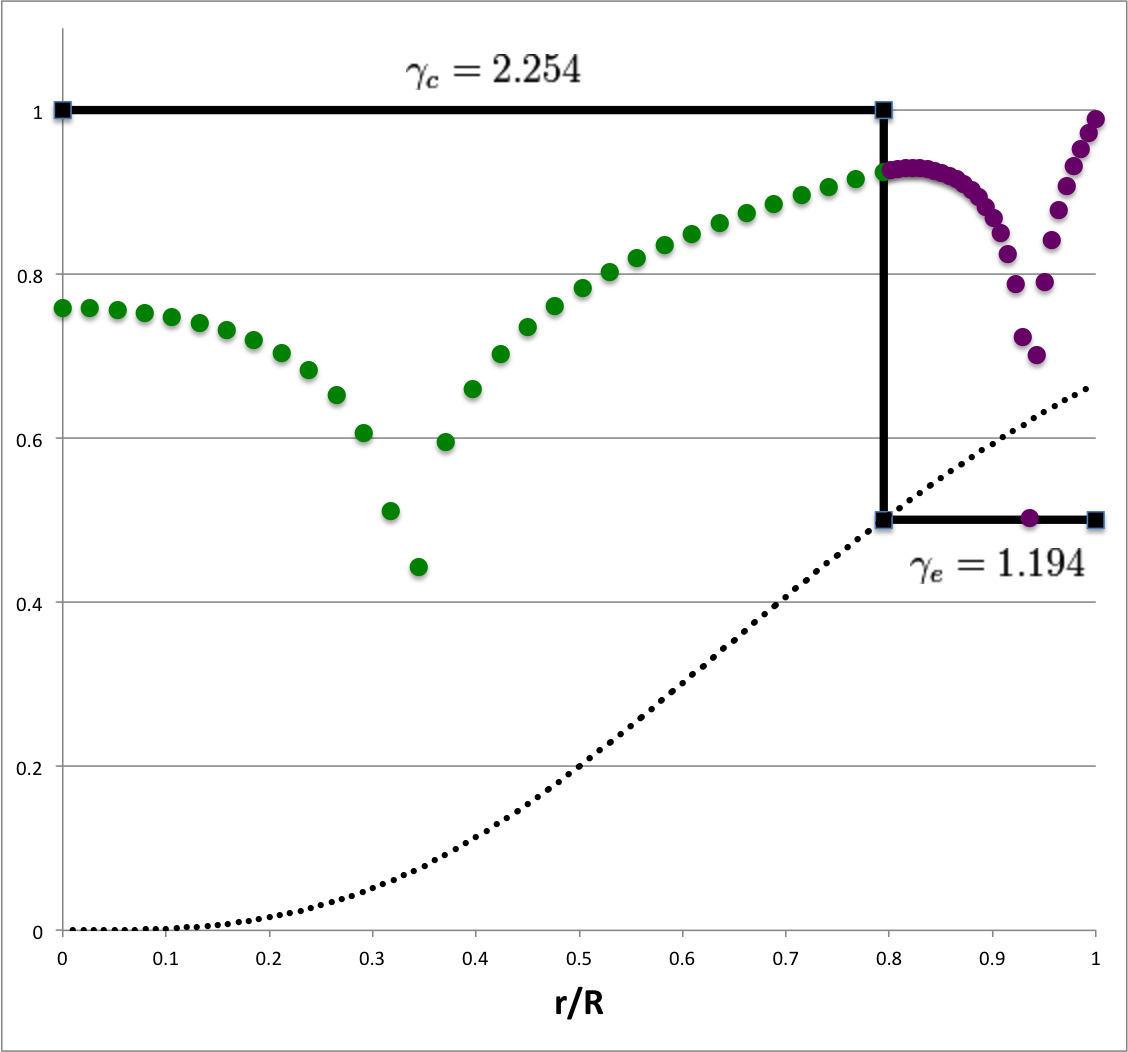
Top-Left Panel: Plotted points show how the location of the core/envelope interface, <math>~q \equiv r_i/R</math>, varies with <math>~\alpha_e \equiv (3-4/\gamma_e)</math> — where <math>~\gamma_e</math> is the adiabatic exponent of the envelope — in equilibrium models that are amenable to analytic modal analysis for quantum numbers, <math>~(\ell,j) = (3,1)</math>. Red (alternatively, blue) markers identify models for which the corresponding value of the adiabatic exponent of the core [see bottom-left panel] falls inside (alternatively, outside) the physically viable range, namely, <math>~1 \le \gamma_c \le \infty</math>. The yellow circular marker identifies the model whose analytically determined eigenfunction is displayed on the right, as an example.
Bottom-Left Panel: Plotted points show how <math>~\alpha_c \equiv (3-4/\gamma_c)</math> varies with <math>~\alpha_e</math> over the physically viable parameter range, <math>~-1 \le \alpha \le 3</math>. Both axes have been flipped so that incompressible models <math>~(\gamma = \infty)</math> lie on the left/bottom while isothermal models <math>~(\gamma =1)</math> lie on the right/top. The core is more compressible than the envelope in models that lie above and to the left of the black-dashed, diagonal line. The yellow circular marker identifies the same example model as it does in the top-left panel.
Top-Right Panel: Displays — as a function of the fractional radius, <math>~r_0/R = q\xi</math> — the analytically determined eigenfunction for the <math>~(\ell,j) = (3,1)</math> mode in the model identified by the yellow circular marker in both left-hand panels, for which,
<math>~q = \biggl[0.01 + 40\biggl( \frac{0.98}{99} \biggr) \biggr] \approx 0.4059596</math>
and, correspondingly, <math>~(c_0, \alpha_e,\alpha_c) = (-1.7832574, -0.3865078, -0.9639245)</math>. Specifically, over the radial interval, <math>~0 \le \xi \le 1</math>, the green markers trace the core's contribution to the combined eigenfunction, namely,
|
<math>~x_{j=1} |_\mathrm{core}</math> |
<math>~=</math> |
<math>~ \frac{5(1+8q^3) - 7 (1+2q^3)^2 \xi^2}{5(1+8q^3)-7(1+2q^3)^2} \, ;</math> |
and, over the radial interval, <math>~1 \le \xi \le 1/q</math>, the purple markers trace the envelope's contribution to the combined eigenfunction, namely,
|
<math>~x_{\ell=3} |_\mathrm{env}</math> |
<math>~=</math> |
<math>~ \xi^{c_0}\biggl[ \frac{ 1 + q^3 A_{31} \xi^{3} + q^6 A_{31}B_{31}\xi^{6} + q^9 A_{31}B_{31}C_{31}\xi^{9} }{ 1 + q^3 A_{31} + q^6 A_{31}B_{31} + q^9 A_{31}B_{31}C_{31} }\biggr] \, , </math> |
where the coefficients, <math>~A_{31}, B_{31}, C_{31}</math>, are as defined above in terms of the parameter, <math>~c_0</math>. The corresponding eigenfrequency is, from the perspective of the core,
|
<math>~\frac{3\omega^2}{2\pi G \rho_c}</math> |
<math>~=</math> |
<math>~20\gamma_c - 8 = \frac{8(7 + \alpha_c)}{3-\alpha_c} \approx 12.18202\, ;</math> |
and, from the perspective of the envelope,
|
<math>~\frac{3\omega^2}{2\pi G \rho_c}</math> |
<math>~=</math> |
<math>~\gamma_e\biggl[2\alpha_e + (c_0 + 9)(c_0+14)\biggr] \frac{\rho_e}{\rho_c} \approx 12.18202\, ,</math> |
where the relevant density ratio is, <math>~\rho_e/\rho_c = 2q^3/(1+2q^3) \approx 0.118016</math>.
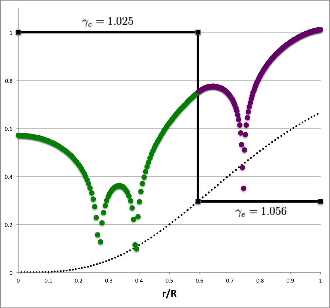
Bottom-Right Panel: The green and purple markers present the same eigenfunction-amplitude information, <math>~x(r/R)</math>, as in the Top-Right panel, but on a logarithmic scale. Specifically, in this plot, the vertical displacement of the green and purple markers is given by the expression,
|
<math>~y</math> |
<math>~=</math> |
<math>~\tfrac{1}{8} \log_{10}[x^2 + \epsilon^2] + y_\mathrm{shift} \, ,</math> |
where, for plotting purposes, we have used, <math>~\epsilon = 10^{-5}</math>, and have set <math>~y_\mathrm{shift}</math> to a value that ensures that <math>~y \approx 1</math> at the outer edge. In this type of log-amplitude plot, the eigenfunction's various nodes — that is, radial locations where <math>~x</math> passes through zero — are highlighted; here, specifically, there is one node inside the core and one node resides in the envelope. Using the vertical coordinate to represent, instead, the configuration's mass-density normalized to its central value, <math>~\rho/\rho_c</math>, the solid black line segments trace the unperturbed density distribution throughout this specific <math>~(n_c, n_e) = (0,0)</math> bipolytrope. Throughout the core, <math>~\rho/\rho_c = 1</math>; then, at the location of the interface <math>~(r_i/R = q \approx 0.41)</math>, the density abruptly drops to its envelope value <math>~(\rho/\rho_c = \rho_e/\rho_c \approx 0.12)</math>.
NOTE: As may be ascertained from our general discussion of the structural properties of <math>~(n_c, n_e) = (0,0)</math> bipolytropes, equilibrium "zero-zero" bipolytropes can be constructed with the envelope/core interface parameter set to any value across the range, <math>~0 \le q \le 1</math>; and for any chosen value of <math>~q</math>, the envelope/core density ratio can, in principle, be set to any value, <math>~0 \le \rho_e/\rho_c \le 1</math>. We have not, however, been able to analytically solve the relevant pair of linear-adiabatic wave equations (LAWEs) for this entire set of equilibrium models. Instead, our ability to derive analytically prescribed eigenvectors is limited by the constraint,
|
<math>~\frac{\rho_e}{\rho_c}</math> |
<math>~=</math> |
<math>~\frac{2q^3}{1+2q^3} = \frac{2(r_i/R)^3}{1+2(r_i/R)^3}\, .</math> |
The black-dotted curve in the Bottom-Right Panel displays the behavior of this constraint; accordingly, the step function depicted by the solid black line segments must necessarily drop from unity to a point on this black-dotted curve for any equilibrium model — such as the example illustrated here — that has an analytically prescribable radial-oscillation eigenvector.
Try Mode32 <math>~(\ell,j) = (3,2)</math>
Setup32
Here, we set the quantum numbers to <math>~(\ell,j) = (3,2)</math>. In this case, as when addessing Mode22, above, the core eigenfunction segment should be,
|
<math>~x_{j=2} |_\mathrm{core}</math> |
<math>~=</math> |
<math>~ \frac{35(1+8q^3)^2 - 126(1+8q^3) (1+2q^3)^2 \xi^2 + 99 (1+2q^3)^4 \xi^4 }{35(1+8q^3)^2 - 126(1+8q^3) (1+2q^3)^2 + 99 (1+2q^3)^4 } \, ;</math> |
and, as when addressing Mode31, above, throughout the envelope, the eigenfunction should be,
|
<math>~x_{\ell=3} |_\mathrm{env}</math> |
<math>~=</math> |
<math>~ \xi^{c_0}\biggl[ \frac{ 1 + q^3 A_{32} \xi^{3} + q^6 A_{32}B_{32}\xi^{6} + q^9 A_{32}B_{32}C_{32}\xi^{9} }{ 1 + q^3 A_{32} + q^6 A_{32}B_{32} + q^9 A_{32}B_{32}C_{32} }\biggr] \, , </math> |
where,
|
<math>~A_{32}</math> |
<math>~=</math> |
<math>~\frac{- 6(c_0 + 7)}{2c_0 + 5 } \, ,</math> |
|
<math>~B_{32}</math> |
<math>~=</math> |
<math>~\frac{ - (6c_0 + 51)}{ 6(c_0 +4) } \, ,</math> |
|
<math>~C_{32}</math> |
<math>~=</math> |
<math>~\frac{- 2( c_0 + 10)}{7( c_0 + 6) } \, .</math> |
In establishing the interface matching conditions, we should be able to follow the same steps as in our search for "31" modes, but replace <math>~Q_{31}</math> with,
|
<math>~Q_{32}</math> |
<math>~\equiv</math> |
<math>~ \frac{ - 252(1+8q^3) (1+2\Chi)^2 + 396 (1+2\Chi)^4 }{35(1+8q^3)^2 - 126(1+8q^3) (1+2q^3)^2 + 99 (1+2q^3)^4 } \, . </math> |
And, in order for the two (dimensional) eigenfrequencies to match, the adiabatic exponent for the core must be,
|
<math>~ \gamma_c </math> |
<math>~=</math> |
<math>~\frac{1}{ 6 + 2j(2j+5)] } \biggl\{ 8 + \gamma_e \biggl[2\alpha_e + (c_0 + 3\ell)(c_0 + 3\ell +5) \biggr]\frac{\rho_e}{\rho_c} \biggr\} </math> |
|
|
<math>~=</math> |
<math>~\frac{1}{42} \biggl\{ 8 + \gamma_e \biggl[2\alpha_e + (c_0 + 9)(c_0 + 14) \biggr]\frac{\rho_e}{\rho_c} \biggr\} \, . </math> |
Illustration32
|
Analytically Definable Eigenvectors in <math>~(n_c, n_e) = (0,0)</math> Bipolytropes Quantum Numbers: <math>~(\ell,j) = (3,2)</math> |
|
|---|---|
| Analyzable Model Sequence | One Example Eigenfunction |
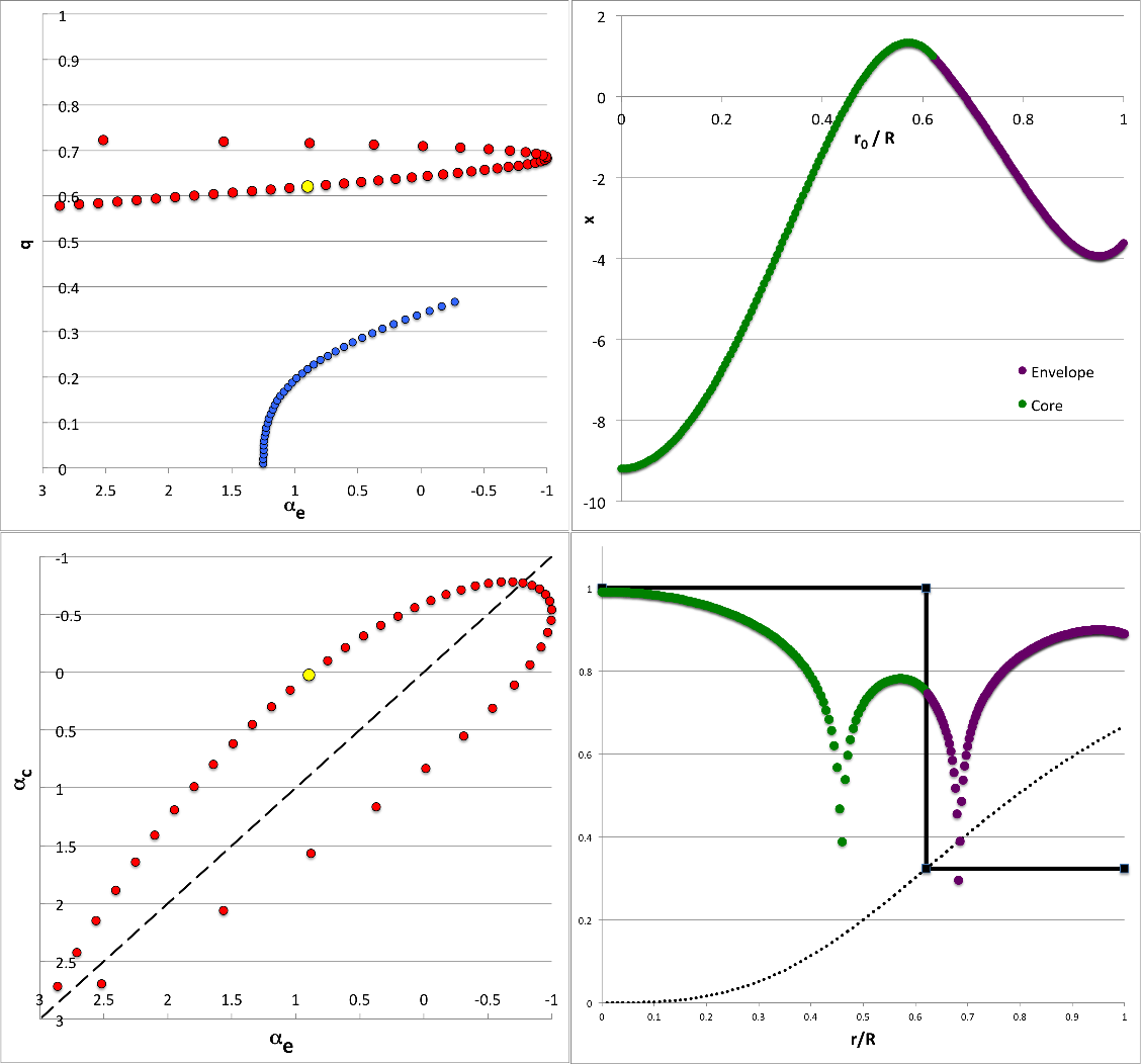
Top-Left Panel: Plotted points show how the location of the core/envelope interface, <math>~q \equiv r_i/R</math>, varies with <math>~\alpha_e \equiv (3-4/\gamma_e)</math> — where <math>~\gamma_e</math> is the adiabatic exponent of the envelope — in equilibrium models that are amenable to analytic modal analysis for quantum numbers, <math>~(\ell,j) = (3,2)</math>. Red (alternatively, blue) markers identify models for which the corresponding value of the adiabatic exponent of the core [see bottom-left panel] falls inside (alternatively, outside) the physically viable range, namely, <math>~1 \le \gamma_c \le \infty</math>. The yellow circular marker identifies the model whose analytically determined eigenfunction is displayed on the right, as an example.
Bottom-Left Panel: Plotted points show how <math>~\alpha_c \equiv (3-4/\gamma_c)</math> varies with <math>~\alpha_e</math> over the physically viable parameter range, <math>~-1 \le \alpha \le 3</math>. Both axes have been flipped so that incompressible models <math>~(\gamma = \infty)</math> lie on the left/bottom while isothermal models <math>~(\gamma =1)</math> lie on the right/top. The core is more compressible than the envelope in models that lie above and to the left of the black-dashed, diagonal line. The yellow circular marker identifies the same example model as it does in the top-left panel.
Top-Right Panel: Displays — as a function of the fractional radius, <math>~r_0/R = q\xi</math> — the analytically determined eigenfunction for the <math>~(\ell,j) = (3,2)</math> mode in the model identified by the yellow circular marker in both left-hand panels, for which,
<math>~q = \biggl[0.01 + 185\biggl( \frac{0.98}{3\times 99} \biggr)\biggr] \approx 0.6204377</math>
and, correspondingly, <math>~(c_0, \alpha_e,\alpha_c) = (-2.3774068, + 0.8972496, +0.0231304)</math>. Specifically, over the radial interval, <math>~0 \le \xi \le 1</math>, the green markers trace the core's contribution to the combined eigenfunction as defined by the expression for <math>~x_{j=2} |_\mathrm{core}</math>, given above; and, over the radial interval, <math>~1 \le \xi \le 1/q</math>, the purple markers trace the envelope's contribution to the combined eigenfunction as defined by the expression for <math>~x_{\ell=3} |_\mathrm{env}</math>, given above.
The corresponding eigenfrequency is, from the perspective of the core,
|
<math>~\frac{3\omega^2}{2\pi G \rho_c}</math> |
<math>~=</math> |
<math>~42\gamma_c - 8 = \frac{8(18 + \alpha_c)}{3-\alpha_c} \approx 48.4351\, ;</math> |
and, from the perspective of the envelope,
|
<math>~\frac{3\omega^2}{2\pi G \rho_c}</math> |
<math>~=</math> |
<math>~\gamma_e\biggl[2\alpha_e + (c_0 + 9)(c_0+14)\biggr] \frac{\rho_e}{\rho_c} \approx 48.4351 \, ,</math> |
where the relevant density ratio is, <math>~\rho_e/\rho_c = 2q^3/(1+2q^3) \approx 0.323257</math>.
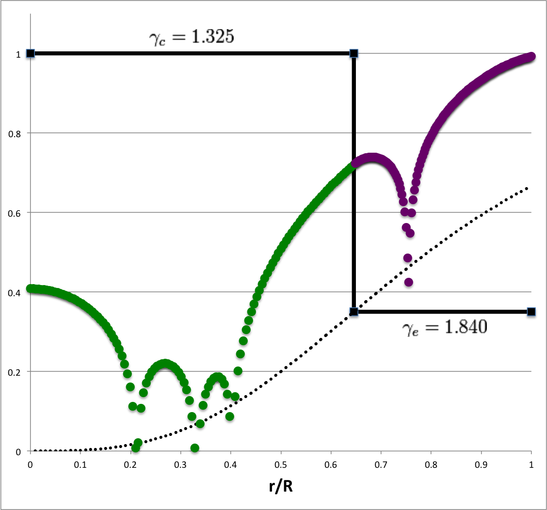
Bottom-Right Panel: The green and purple markers present the same eigenfunction-amplitude information, <math>~x(r/R)</math>, as in the Top-Right panel, but on a logarithmic scale. Specifically, in this plot, the vertical displacement of the green and purple markers is given by the expression,
|
<math>~y</math> |
<math>~=</math> |
<math>~\tfrac{1}{8} \log_{10}[x^2 + \epsilon^2] + y_\mathrm{shift} \, ,</math> |
where, for plotting purposes, we have used, <math>~\epsilon = 10^{-5}</math>, and have set <math>~y_\mathrm{shift}</math> to a value that ensures that <math>~y \approx 1</math> at the enter of the configuration. In this type of log-amplitude plot, the eigenfunction's various nodes — that is, radial locations where <math>~x</math> passes through zero — are highlighted; here, specifically, there is one node inside the core and one node resides in the envelope. Using the vertical coordinate to represent, instead, the configuration's mass-density normalized to its central value, <math>~\rho/\rho_c</math>, the solid black line segments trace the unperturbed density distribution throughout this specific <math>~(n_c, n_e) = (0,0)</math> bipolytrope. Throughout the core, <math>~\rho/\rho_c = 1</math>; then, at the location of the interface <math>~(r_i/R = q \approx 0.62)</math>, the density abruptly drops to its envelope value <math>~(\rho/\rho_c = \rho_e/\rho_c \approx 0.32)</math>.
NOTE: As may be ascertained from our general discussion of the structural properties of <math>~(n_c, n_e) = (0,0)</math> bipolytropes, equilibrium "zero-zero" bipolytropes can be constructed with the envelope/core interface parameter set to any value across the range, <math>~0 \le q \le 1</math>; and for any chosen value of <math>~q</math>, the envelope/core density ratio can, in principle, be set to any value, <math>~0 \le \rho_e/\rho_c \le 1</math>. We have not, however, been able to analytically solve the relevant pair of linear-adiabatic wave equations (LAWEs) for this entire set of equilibrium models. Instead, our ability to derive analytically prescribed eigenvectors is limited by the constraint,
|
<math>~\frac{\rho_e}{\rho_c}</math> |
<math>~=</math> |
<math>~\frac{2q^3}{1+2q^3} = \frac{2(r_i/R)^3}{1+2(r_i/R)^3}\, .</math> |
The black-dotted curve in the Bottom-Right Panel displays the behavior of this constraint; accordingly, the step function depicted by the solid black line segments must necessarily drop from unity to a point on this black-dotted curve for any equilibrium model — such as the example illustrated here — that has an analytically prescribable radial-oscillation eigenvector.
Try Mode33 <math>~(\ell,j) = (3,3)</math>
Setup33
Here, we set the quantum numbers to <math>~(\ell,j) = (3,3)</math>. In this case, drawing from our summary of Sterne's presentation, the core eigenfunction segment should be,
|
<math>~x_{j=3} |_\mathrm{core}</math> |
<math>~=</math> |
<math>~ \frac{3\cdot 5 \cdot 7 - 33\cdot 3\cdot 7 (1+2q^3)^2 \xi^2 + 429\cdot 3 (1+2q^3)^4 \xi^4 - 143\cdot 5 (1+2q^3)^6 \xi^6}{3\cdot 5 \cdot 7 - 33\cdot 3\cdot 7 (1+2q^3)^2 + 429\cdot 3 (1+2q^3)^4 - 143\cdot 5 (1+2q^3)^6 } \, ,</math> |
and, as when addressing Mode31, above, throughout the envelope, the eigenfunction should be,
|
<math>~x_{\ell=3} |_\mathrm{env}</math> |
<math>~=</math> |
<math>~ \xi^{c_0}\biggl[ \frac{ 1 + q^3 A_{33} \xi^{3} + q^6 A_{33}B_{33}\xi^{6} + q^9 A_{33}B_{33}C_{33}\xi^{9} }{ 1 + q^3 A_{33} + q^6 A_{33}B_{33} + q^9 A_{33}B_{33}C_{33} }\biggr] \, , </math> |
where,
|
<math>~A_{33}</math> |
<math>~=</math> |
<math>~\frac{- 6(c_0 + 7)}{2c_0 + 5 } \, ,</math> |
|
<math>~B_{33}</math> |
<math>~=</math> |
<math>~\frac{ - (6c_0 + 51)}{ 6(c_0 +4) } \, ,</math> |
|
<math>~C_{33}</math> |
<math>~=</math> |
<math>~\frac{- 2( c_0 + 10)}{7( c_0 + 6) } \, .</math> |
In establishing the interface matching conditions, we should be able to follow the same steps as in our search for "31" modes, but replace <math>~Q_{31}</math> with,
|
<math>~Q_{33}</math> |
<math>~\equiv</math> |
<math>~ \frac{ - 2\cdot 33\cdot 3\cdot 7 (1+2q^3)^2 + 4\cdot 429\cdot 3 (1+2q^3)^4 - 6\cdot 143\cdot 5 (1+2q^3)^6 }{3\cdot 5 \cdot 7 - 33\cdot 3\cdot 7 (1+2q^3)^2 + 429\cdot 3 (1+2q^3)^4 - 143\cdot 5 (1+2q^3)^6 } \, . </math> |
And, in order for the two (dimensional) eigenfrequencies to match, the adiabatic exponent for the core must be,
|
<math>~ \gamma_c </math> |
<math>~=</math> |
<math>~\frac{1}{ 6 + 2j(2j+5)] } \biggl\{ 8 + \gamma_e \biggl[2\alpha_e + (c_0 + 3\ell)(c_0 + 3\ell +5) \biggr]\frac{\rho_e}{\rho_c} \biggr\} </math> |
|
|
<math>~=</math> |
<math>~\frac{1}{72} \biggl\{ 8 + \gamma_e \biggl[2\alpha_e + (c_0 + 9)(c_0 + 14) \biggr]\frac{\rho_e}{\rho_c} \biggr\} \, . </math> |
| Figure 4: Results for mode <math>~(\ell,j) = (3,3)</math> | ||
|
[[|850px|Results for (ell,j) = (3,3)]] |
<math>~q</math> | <math>~ </math> |
| <math>~c_0</math> | <math>~ </math> | |
| <math>~\gamma_e</math> | <math>~ </math> | |
| <math>~\alpha_e</math> | <math>~0. </math> | |
| <math>~n_e</math> | <math>~ </math> | |
| <math>~\nu</math> | <math>~ </math> | |
| <math>~\rho_e/\rho_c</math> | <math>~ </math> | |
| <math>~\gamma_c</math> | <math>~ </math> | |
| <math>~\alpha_c</math> | <math>~ </math> | |
Illustration33
|
Analytically Definable Eigenvectors in <math>~(n_c, n_e) = (0,0)</math> Bipolytropes Quantum Numbers: <math>~(\ell,j) = (3,3)</math> |
|
|---|---|
| Analyzable Model Sequence | One Example Eigenfunction |
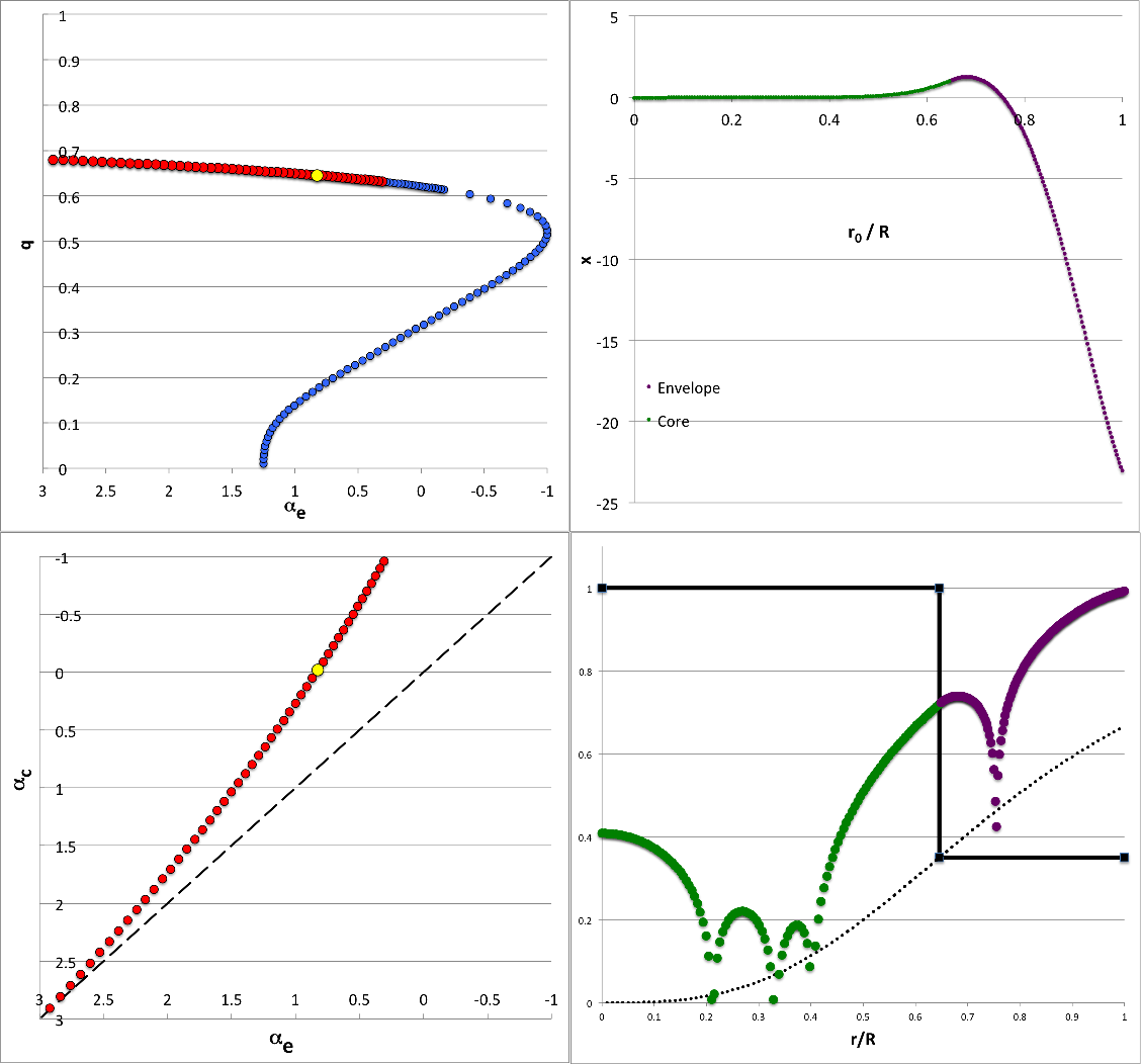
Top-Left Panel: Plotted points show how the location of the core/envelope interface, <math>~q \equiv r_i/R</math>, varies with <math>~\alpha_e \equiv (3-4/\gamma_e)</math> — where <math>~\gamma_e</math> is the adiabatic exponent of the envelope — in equilibrium models that are amenable to analytic modal analysis for quantum numbers, <math>~(\ell,j) = (3,3)</math>. Red (alternatively, blue) markers identify models for which the corresponding value of the adiabatic exponent of the core [see bottom-left panel] falls inside (alternatively, outside) the physically viable range, namely, <math>~1 \le \gamma_c \le \infty</math>. The yellow circular marker identifies the model whose analytically determined eigenfunction is displayed on the right, as an example.
Bottom-Left Panel: Plotted points show how <math>~\alpha_c \equiv (3-4/\gamma_c)</math> varies with <math>~\alpha_e</math> over the physically viable parameter range, <math>~-1 \le \alpha \le 3</math>. Both axes have been flipped so that incompressible models <math>~(\gamma = \infty)</math> lie on the left/bottom while isothermal models <math>~(\gamma =1)</math> lie on the right/top. The core is more compressible than the envelope in models that lie above and to the left of the black-dashed, diagonal line. The yellow circular marker identifies the same example model as it does in the top-left panel.
Top-Right Panel: Displays — as a function of the fractional radius, <math>~r_0/R = q\xi</math> — the analytically determined eigenfunction for the <math>~(\ell,j) = (3,2)</math> mode in the model identified by the yellow circular marker in both left-hand panels, for which,
<math>~q = 0.01 + 642\biggl( \frac{0.98}{990} \biggr) \approx 0.6455152 \, ,</math>
and, correspondingly, <math>~(c_0, \alpha_e,\alpha_c) = (+0.3511525, +0.8256130, -0.0183637)</math>. Specifically, over the radial interval, <math>~0 \le \xi \le 1</math>, the green markers trace the core's contribution to the combined eigenfunction as defined by the expression for <math>~x_{j=3} |_\mathrm{core}</math>, given above; and, over the radial interval, <math>~1 \le \xi \le 1/q</math>, the purple markers trace the envelope's contribution to the combined eigenfunction as defined by the expression for <math>~x_{\ell=3} |_\mathrm{env}</math>, given above.
The corresponding eigenfrequency is, from the perspective of the core,
|
<math>~\frac{3\omega^2}{2\pi G \rho_c}</math> |
<math>~=</math> |
<math>~72\gamma_c - 8 = \frac{8(33 + \alpha_c)}{3-\alpha_c} \approx 87.41594 \, ;</math> |
and, from the perspective of the envelope,
|
<math>~\frac{3\omega^2}{2\pi G \rho_c}</math> |
<math>~=</math> |
<math>~\gamma_e\biggl[2\alpha_e + (c_0 + 9)(c_0+14)\biggr] \frac{\rho_e}{\rho_c} \approx 87.41594 \, ,</math> |
where the relevant density ratio is, <math>~\rho_e/\rho_c = 2q^3/(1+2q^3) \approx 0.3497877</math>.
Bottom-Right Panel: The green and purple markers present the same eigenfunction-amplitude information, <math>~x(r/R)</math>, as in the Top-Right panel, but on a logarithmic scale. Specifically, in this plot, the vertical displacement of the green and purple markers is given by the expression,
|
<math>~y</math> |
<math>~=</math> |
<math>~\tfrac{1}{10} \log_{10}[x^2 + \epsilon^2] + y_\mathrm{shift} \, ,</math> |
where, for plotting purposes, we have used, <math>~\epsilon = 10^{-5}</math>, and have set <math>~y_\mathrm{shift}</math> to a value that ensures that <math>~y \approx 1</math> at the outer edge. In this type of log-amplitude plot, the eigenfunction's various nodes — that is, radial locations where <math>~x</math> passes through zero — are highlighted; here, specifically, there are three nodes inside the core and one node resides in the envelope. Using the vertical coordinate to represent, instead, the configuration's mass-density normalized to its central value, <math>~\rho/\rho_c</math>, the solid black line segments trace the unperturbed density distribution throughout this specific <math>~(n_c, n_e) = (0,0)</math> bipolytrope. Throughout the core, <math>~\rho/\rho_c = 1</math>; then, at the location of the interface <math>~(r_i/R = q \approx 0.65)</math>, the density abruptly drops to its envelope value <math>~(\rho/\rho_c = \rho_e/\rho_c \approx 0.35)</math>.
NOTE: As may be ascertained from our general discussion of the structural properties of <math>~(n_c, n_e) = (0,0)</math> bipolytropes, equilibrium "zero-zero" bipolytropes can be constructed with the envelope/core interface parameter set to any value across the range, <math>~0 \le q \le 1</math>; and for any chosen value of <math>~q</math>, the envelope/core density ratio can, in principle, be set to any value, <math>~0 \le \rho_e/\rho_c \le 1</math>. We have not, however, been able to analytically solve the relevant pair of linear-adiabatic wave equations (LAWEs) for this entire set of equilibrium models. Instead, our ability to derive analytically prescribed eigenvectors is limited by the constraint,
|
<math>~\frac{\rho_e}{\rho_c}</math> |
<math>~=</math> |
<math>~\frac{2q^3}{1+2q^3} = \frac{2(r_i/R)^3}{1+2(r_i/R)^3}\, .</math> |
The black-dotted curve in the Bottom-Right Panel displays the behavior of this constraint; accordingly, the step function depicted by the solid black line segments must necessarily drop from unity to a point on this black-dotted curve for any equilibrium model — such as the example illustrated here — that has an analytically prescribable radial-oscillation eigenvector.
Summary Plots
Related Discussions

|
|---|
|
© 2014 - 2021 by Joel E. Tohline |
