Summary for Hadley & Imamura

This MediaWiki-based document is especially provided for Jimmy Imamura and Kathryn Hadley. It summarizes the contents of a much longer set of technical notes that discusses the analysis of nonaxisymmetric distortions in rotating, self-gravitating fluids. The punchline is provided by the animation sequence shown in Figure 2, below.

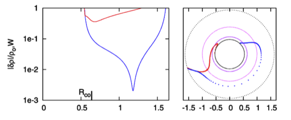
While studying the series of three papers that has recently been published by the Imamura & Hadley collaboration, I was particularly drawn to the pair of plots presented in Figure 6 — and, again, in the top portion of Figure 13 and the top portion of Figure 16 — of HI11. This pair of plots has been reprinted here, without modification, as our Figure 1. The curves delineated by the blue dots in this pair of HI11 plots display (on the left) the shape of the eigenfunction, <math>~f_1(\varpi)</math>, and (on the right) the "constant phase loci," <math>~\phi_1(\varpi)</math>, for an unstable, <math>~m=1</math> mode. In this case, the initial model for the depicted evolution is the equilibrium model from Table 2 of HI11 that has <math>~T/|W| = 0.253</math>; it is a fully self-gravitating torus with polytropic index, <math>~n = 3/2</math>, and a rotation-law profile defined by a "Keplerian" angular velocity profile.

Figure 1

Panel pair extracted^† without modification from the top-most segment of Figure 13, p. 18 of K. Hadley & J. N. Imamura (2011)

"Nonaxisymmetric Instabilities of Self-Gravitating Disks. I Toroids"

Astrophysics and Space Science, 334, 1 - 26 © Springer Science+Business Media B.V.

^†This pair of plots also appears in the top portion of Figure 16 on p. 20 and, by itself, as Figure 6 on p. 12 of K. Hadley & J. N. Imamura (2011).

Radial Eigenfunction

Recognition #1

It occurred to me, first, that the blue curve displayed in the left-hand panel of Figure 1 might be reasonably well approximated by piecing together a pair of arc-hyperbolic-tangent (ATANH) functions. In an effort to demonstrate this, I began by specifying a "midway" radial location, <math>~r_- < r_\mathrm{mid} < r_+ \, ,</math> at which the two ATANH functions meet and at which the density fluctuation is smallest. Then I defined a function of the form,

	<math>~f_\ln(\varpi)</math>	<math>~=</math>	<math>~\tanh^{-1}\biggl[1 - 2 \biggl( \frac{\varpi - r_-}{r_\mathrm{mid}-r_-} \biggr) \biggr]</math>	for	<math>r_- < \varpi < r_\mathrm{mid} \, ;</math>
and
	<math>~f_\ln(\varpi)</math>	<math>~=</math>	<math>~\tanh^{-1}\biggl[1 - 2 \biggl( \frac{\varpi - r_+}{r_\mathrm{mid}-r_+} \biggr) \biggr]</math>	for	<math>r_\mathrm{mid} < \varpi < r_+ \, .</math>

Recognizing that the figure depicting the HI11 eigenfunction is a semi-log plot, it seems clear that the relationship between our constructed function, <math>~f_\ln(\varpi)</math>, and the eigenfunction, <math>~f_1(\varpi)</math>, is,

<math>~f_1(\varpi) = e^{f_\ln(\varpi)} \, .</math>

Recognition #2

Given that, in general, the following mathematical relation holds,

<math>~\ln\biggl( \frac{1+x}{1-x} \biggr)^{1/2} </math>

for

we can write for the innermost region of the toroidal configuration — that is, over the lower radial-coordinate range —

<math>~f_1(\varpi) = e^{f_\ln(\varpi)}</math>

<math>~\biggl( \frac{r_\mathrm{mid} - \varpi}{\varpi - r_-} \biggr)^{1/2} </math>

for

Similarly, we find that, over the upper radial-coordinate range,

<math>~f_1(\varpi) = e^{f_\ln(\varpi)}</math>

<math>~\biggl( \frac{r_\mathrm{mid} - \varpi}{\varpi - r_+} \biggr)^{1/2} </math>

for

<math>r_\mathrm{mid} < \varpi < r_+ \, .</math>

Recognition #3

After a bit more experimentation, we recognized that it is advantageous to replace the square root — that is, the exponent, ½ — with a variable exponent, <math>~p</math>, that can serve as an adjustable fitting parameter; and, in order to facilitate a degree of radial overlap between the two ATANH functions, we introduced different values of <math>~r_\mathrm{mid}</math> on the left and on the right. This led to a two-piece radial eigenfunction of the form,

<math>~f_\mathrm{blue}(\varpi) </math>

<math>~\biggl( \frac{r_\mathrm{blue} - \varpi}{\varpi - r_-} \biggr)^{p} </math>

for

<math>r_- < \varpi < r_\mathrm{blue} </math> … <math>~\biggl[ f_\mathrm{blue}(\varpi) = 0</math> otherwise<math>~\biggr]</math>,

and,

<math>~f_\mathrm{green}(\varpi) </math>

<math>~\biggl( \frac{r_\mathrm{green} - \varpi}{\varpi - r_+} \biggr)^{p} </math>

for

<math>r_\mathrm{green} < \varpi < r_+ </math> … <math>~\biggl[ f_\mathrm{green}(\varpi) = 0</math> otherwise<math>~\biggr]</math>,

where, <math>~r_\mathrm{mid}|_\mathrm{green} \le r_\mathrm{mid}|_\mathrm{blue}</math>.

Summary

The expression that we are currently using for the radial eigenfunction is a sum of these two pieces, that is,

<math>~f_1(\varpi)</math>

<math>~f_\mathrm{green}(\varpi) + f_\mathrm{blue}(\varpi) \, . </math>

For later use, we define from this function the minimum and maximum values,

<math>~[f_\ln]_\mathrm{min} \equiv \mathrm{min}[\ln(f_1)]</math>

and

<math>~[f_\ln]_\mathrm{max} \equiv \mathrm{max}[\ln(f_1)] \, .</math>

Constant Phase Loci

As is explained in our accompanying detailed technical notes — see, also another improvement — we have settled on the following prescription for the phase function, <math>~\phi_m(\varpi)</math>:

<math>~\pm \tan^{-1}[\aleph_m \cdot D_{1/2}(\varpi)] \, .</math>

where,

<math>~D_{1/2}(\varpi)</math>

<math>~\equiv</math>

<math>~\biggl[ \frac{f_\ln(\varpi) - [f_\ln]_\mathrm{min}}{[f_\ln]_\mathrm{max} - [f_\ln]_\mathrm{min}} \biggr]^{1/2} \, ,</math>

<math>~\aleph_m</math> is a (perhaps, mode-dependent) constant to be specified, and,

<math>~f_\ln(\varpi)</math>

<math>~\equiv</math>

<math>~\ln[ f_1(\varpi)] \, .</math>

Put It Together

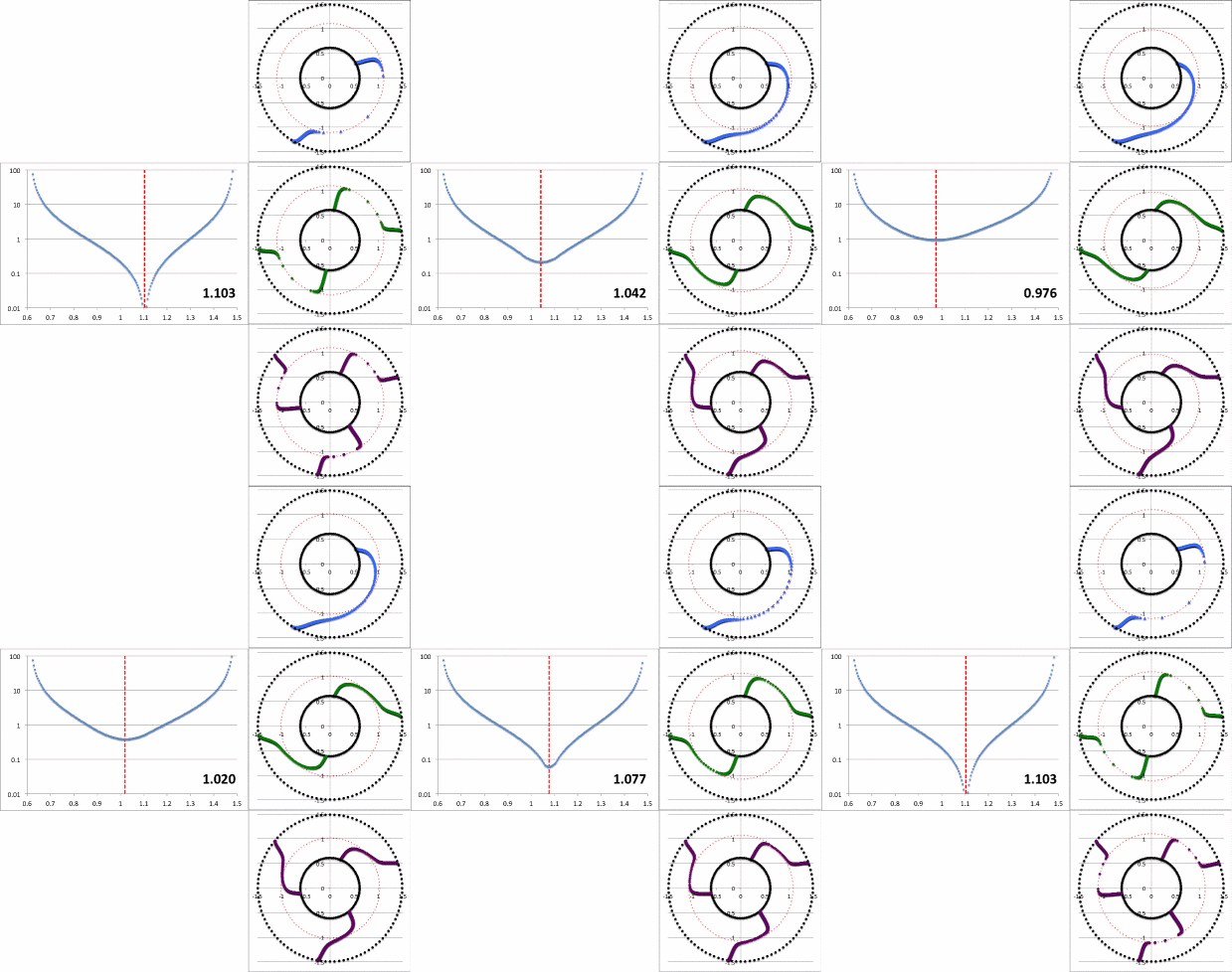
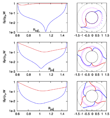
Figure 2a contains an animation sequence that is intended to illustrate that our empirically constructed radial eigenfunction and accompanying polar-coordinate plots of "constant phase loci" closely resemble the radial eigenfunctions and constant phase loci that have been displayed in HI11's Figure 16 (a portion of which is redisplayed, here, as Figure 2b). Each frame of the Figure 2a animation, contains (on the left) a semi-log plot of <math>~f_1(\varpi)</math> versus <math>~\varpi</math> and (on the right) the corresponding constant phase loci that are generated for <math>~\phi_1</math> (top), <math>~\phi_2</math> (middle), and <math>~\phi_3</math> (bottom), when the natural log of the same function, <math>~f_\ln = \ln[f_1(\varpi)]</math>, is plugged into our empirically derived function, <math>~D_{1/2}</math>. In a separate chapter we demonstrate in more detail how each frame of this animation sequence was constructed. As displayed in Figure 2a, <math>~r_\mathrm{green}</math> is the only parameter that is varied from frame to frame of the animation (the seven specified values are listed in a column to the left of the animation); all of the other empirical model parameters — <math>~r_\mathrm{blue}</math>, <math>~p</math>, and <math>~\aleph_m</math> — are held fixed.

Figure 2: Radial and Azimuthal Eigenfunction Comparison

(a) Our Empirically Constructed Function

(b) Extracted from Figure 16 of HI11

Specified <math>~r_\mathrm{green}</math>	Resulting <math>~r_\mathrm{min}</math>
1.10324	1.103
1.05929	1.077
1.01534	1.059
0.97139	1.042
0.88349	1.020
0.75164	0.998
0.61979	0.976

Notice that, by simply varying the value of <math>~r_\mathrm{green}</math>, our semi-log plot of <math>~f_1</math> versus <math>~\varpi</math> sweeps through shapes that qualitatively match the three radial eigenfunctions (see Figure 2b) that arose in the HI11 investigation. At the largest value, <math>~r_\mathrm{green} = 1.10324</math> (1^st frame of the animation loop), the minimum of the radial eigenfunction is sharply defined and sits at <math>~r_\mathrm{min} = 1.103</math>, as labeled in the animation; the <math>~f_1(\varpi)</math> eigenfunction displayed in this particular frame closely resembles the radial eigenfunction shown at the top of the HI11 figure and, simultaneously, the <math>~m=1</math> constant phase loci plot that appears in the same frame of the animation closely resembles the <math>~m=1</math> constant phase loci plot that is displayed at the top of the HI11 figure. When we set <math>~r_\mathrm{green} = 1.05929</math> (2^nd frame of the animation), the minimum of the radial eigenfunction is still well-defined and sits at <math>~r_\mathrm{min} = 1.077</math>, as labeled in the animation. The <math>~f_1(\varpi)</math> eigenfunction displayed in this 2^nd frame closely resembles the radial eigenfunction shown in the middle panel of the HI11 figure and, simultaneously, the <math>~m=2</math> constant phase loci plot that appears in this 2^nd frame of the animation closely resembles the <math>~m=2</math> constant phase loci plot that is displayed at the middle of the HI11 figure.

Additional Comments

I was delighted to be able to find a single function, such as <math>f_\ln = \ln[f_1(\varpi)]</math>, that can pretty faithfully represent, not just one, but a set of HI11's observed eigenfunctions by simply adjusting one parameter, <math>~f_\mathrm{green}</math>. I was quite happy with this finding and, originally, had no expectation that the function, <math>~f_\ln</math>, would in any way relate to the functional behavior of the corresponding "constant phase loci." After all, it seemed to me that, in general, one should expect that an eigenvector's "amplitude" and "phase" functions will be totally independent of one another.
I was extraordinarily pleased — and stunned! — to find that the same function, <math>~f_\ln</math>, also could be used to provide a reasonably faithful representation of the phase function, <math>~\phi(\varpi)</math>.
In retrospect, it seems clear that the pairs of "amplitude" and "phase" plots published by HI11 for various unstable eigenmodes do exhibit a strong degree of interdependence:
1. The radial location, <math>~r_\mathrm{min}</math>, at which the "amplitude" plot exhibits a minimum (identified, for example, by the red, vertical, dashed line in our Figure 2a animation) also appears to be the radial location at which the "phase" plot exhibits a rapid phase swing (identified by the red, dashed circle in our Figure 2a animation).
2. The degree to which a given "constant phase loci" exhibits a rapid phase swing appears to correlate with the steepness of the <math>~f_\ln(\varpi)</math> function. If the "amplitude" plot exhibits a sharp, well-defined minimum, then the "phase" plot exhibits a sharp phase swing; conversely, if the "amplitude" plot is rather smooth and featureless, then the "phase" plot exhibits milder phase swings.

User:Tohline/Appendix/Ramblings/To Hadley and Imamura

Contents