Analyzing Azimuthal Distortions

In what follows, we will draw heavily from three publications: (1) J. E. Tohline & I. Hachisu (1990, ApJ, 361, 394-407) — hereafter, TH90 — (2) J. W. Woodward, J. E. Tohline, & I. Hachisu (1994, ApJ, 420, 247-267) — hereafter, WTH94 — and (3) K. Hadley & J. N. Imamura (2011, Astrophysics and Space Science, 334, 1) — hereafter, HI11.

Adopted Notation

Beginning with equation (2) of TH90 but ignoring variations in the vertical coordinate direction, the mass density is given by the expression,

<math>~\rho_0 \biggl[ 1 + f(\varpi)e^{-i(\omega t - m\phi)} \biggr] \, ,</math>

where it is understood that <math>~\rho_0</math>, which defines the structure of the initial axisymmetric equilibrium configuration, is generally a function of the cylindrical radial coordinate, <math>~\varpi</math>.

Using the subscript, <math>~m</math>, to identify the time-invariant coefficients and functions that characterize the intrinsic eigenvector of each azimuthal eigen-mode, and acknowledging that the associated eigenfrequency will in general be imaginary, that is,

<math>~\omega_m</math>

<math>~\omega_R + i\omega_I \, ,</math>

we expect each unstable mode to display the following behavior:

<math>~\biggl[ \frac{\rho}{\rho_0} - 1 \biggr]</math>	<math>~=</math>	<math>~f_m(\varpi)e^{-i[\omega_R t + i \omega_I t - m\phi_m(\varpi)]} </math>
	<math>~=</math>	<math>~\biggl\{ f_m(\varpi)e^{-im\phi_m(\varpi)}\biggr\} e^{-i\omega_R t } \cdot e^{\omega_I t} </math>
	<math>~=</math>	<math>~\biggl\{ f_m(\varpi)e^{-i[\omega_R t + m\phi_m(\varpi)]} \biggr\} e^{\omega_I t} \, .</math>

Adopting Kojima's (1986) notation, that is, defining,

<math>~y_1 \equiv \frac{\omega_R}{\Omega_0} - m</math>

and

<math>~y_2 \equiv \frac{\omega_I}{\Omega_0} \, ,</math>

the eigenvector's behavior can furthermore be described by the expression,

<math>~\biggl[ \frac{\rho}{\rho_0} - 1 \biggr]</math>	<math>~=</math>	<math>~\biggl\{ f_m(\varpi)e^{-i[(y_1+m) (\Omega_0 t) + m\phi_m(\varpi)]} \biggr\} e^{y_2 (\Omega_0 t)} </math>
	<math>~=</math>	<math>~\biggl\{ f_m(\varpi)e^{-im[(y_1/m+1) (\Omega_0 t) + \phi_m(\varpi)]} \biggr\} e^{y_2 (\Omega_0 t)} \, .</math>

Note that, as viewed from a frame of reference that is rotating with the mode pattern frequency,

<math>\Omega_p \equiv \frac{\omega_R}{m} = \Omega_0\biggl(\frac{y_1}{m}+1\biggr) \, ,</math>

we should find an eigenvector of the form,

<math>~\biggl[ \frac{\delta\rho}{\rho_0}\biggr]_\mathrm{rot} \equiv \biggl[ \frac{\rho}{\rho_0} - 1 \biggr]e^{im\Omega_p t}</math>

<math>~\biggl\{ f_m(\varpi)e^{-im[\phi_m(\varpi)]} \biggr\} e^{y_2 (\Omega_0 t)} \, ,</math>

whose relative amplitude — with a radial structure as specified inside the curly braces — is undergoing a uniform exponential growth but is otherwise unchanging.

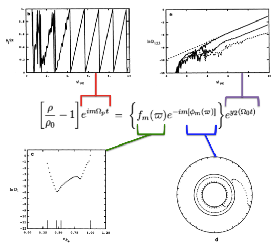
Drawing from figure 2 of WTH94, our Figure 1, immediately below, illustrates how the behavior of each factor in this expression can reveal itself during a numerical simulation that follows the time-evolutionary development of an unstable, nonaxisymmetric eigenmode. The initial model for this depicted evolution (model O3 from Table 1 of WTH94) is a zero-mass — that is, it is a Papaloizou-Pringle like torus — with polytropic index,<math>~n = 3</math>, and a rotation-law profile defined by uniform specific angular momentum.

The top-left panel shows how, at any radial location, the phase angle, <math>~\phi_1/(2\pi)</math>, for the <math>~m=1</math> eigenmode, varies with time, <math>~t/t_\mathrm{rot}</math>, where, <math>~t_\mathrm{rot} \equiv 2\pi/\Omega_0</math> is the rotation period at the density maximum;
Using a semi-log plot, the top-right panel shows the exponential growth of the amplitude of three separate modes: The dominant unstable mode, displaying the largest amplitude, is <math>~m = 1</math>.
Using a semi-log plot (log amplitude versus fractional radius, <math>~\varpi/r_+</math>), the bottom-left panel displays the shape of the eigenfunction, <math>~f_1(\varpi)</math>, for the unstable, <math>~m=1</math> mode;
The bottom-right panel displays the radial dependence of the equatorial-plane phase angle, <math>~\phi_1(\varpi)</math>, for the unstable, <math>~m=1</math> mode; this is what HI11 refer to as the "constant phase loci."

Figure 1

Four panels extracted^† from figure 2, p. 252 of J. W. Woodward, J. E. Tohline & I. Hachisu (1994)

"The Stability of Thick, Self-gravitating Disks in Protostellar Systems"

ApJ, vol. 420, pp. 247-267 © American Astronomical Society

^†As displayed here, the layout of figure panels (a, b, c, d) has been modified from the original publication layout; otherwise, each panel is unmodified.

Empirical Construction of Eigenvector

Summary

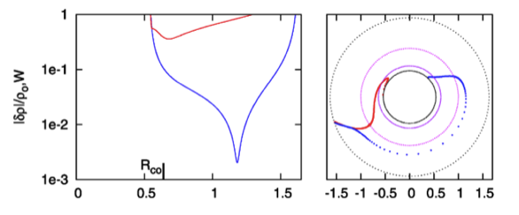
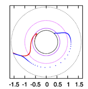
While studying the series of three papers that was published recently by the Imamura & Hadley collaboration, I was particularly drawn to the pair of plots presented in Figure 6 — and, again, in the top portion of Figure 13 — of HI11. This pair of plots has been reprinted here, without modification, as our Figure 2. As in the bottom two panels of our Figure 1, the curves delineated by the blue dots in this pair of HI11 plots display (on the left) the shape of the eigenfunction, <math>~f_1(\varpi)</math>, and (on the right) the "constant phase loci," <math>~\phi_1(\varpi)</math>, for an unstable, <math>~m=1</math> mode. In this case, the initial model for the depicted evolution is the equilibrium model from Table 2 of HI11 that has <math>~T/|W| = 0.253</math>; it is a fully self-gravitating torus with polytropic index, <math>~n = 3/2</math>, and a rotation-law profile defined by a "Keplerian" angular velocity profile.

Figure 2

Panel pair extracted^† without modification from the top-most segment of Figure 13, p. 12 of K. Hadley & J. N. Imamura (2011)

"Nonaxisymmetric Instabilities of Self-Gravitating Disks. I Toroids"

Astrophysics and Space Science, 334, 1 - 26 © Springer Science+Business Media B.V.

^†This pair of plots also appears, by itself, as Figure 6 on p. 12 of K. Hadley & J. N. Imamura (2011).

Figure 3: Our Empirically Constructed Eigenvector

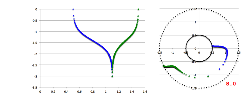
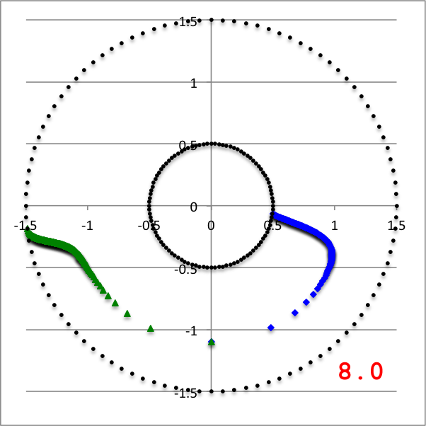
Left panel: A plot of our empirically constructed radial amplitude function, <math>~f_\ln(\varpi)</math>; the function has been normalized as explained in the boxed-in PRACTICAL IMPLEMENTATION remark, below. Right panel: A plot of our empirically constructed phase function, <math>~\phi_1(\varpi)</math> with <math>~\aleph = 8.0</math>; after extraction from the animation sequence presented in Figure 4, here each point along this "constant phase loci" has been shifted by an additional phase of <math>~\pi/10</math> in order to better highlight its resemblance to the HI11 "constant phase loci" plot shown in the righthand panel of our Figure 2. In both panels, blue dots trace the function's behavior over the inner region of the torus <math>~(r_- < \varpi < r_\mathrm{mid})</math> and green dots trace the function's behavior over the outer region of the torus <math>~(r_\mathrm{mid} < \varpi < r_+)</math>.

As is described in the subsections that follow, we have devised two related and relatively simple analytic expressions whose behaviors, as a function of <math>~\varpi</math>, qualitatively resemble the two blue, HI11 curves. Our two empirically constructed functions have been plotted in Figure 3, immediately below Figure 2, to aid visual comparison with the eigenfunctions that were generated by HI11 via a proper stability analysis. Next we describe the thought process that led to the construction of the amplitude and phase eigenfunctions presented in Figure 3.

Radial Eigenfunction

It occurred to me, first, that the blue curve displayed in the left-hand panel of HI11's figure 6 (our Figure 2) might be reasonably well approximated by piecing together a pair of arc-hyperbolic-tangent (ATANH) functions. In an effort to demonstrate this, I began by specifying a "midway" radial location, <math>~r_- < r_\mathrm{mid} < r_+ \, ,</math> at which the two ATANH functions meet and at which the density fluctuation is smallest. Then I defined a function of the form,

	<math>~f_\ln(\varpi)</math>	<math>~=</math>	<math>~\tanh^{-1}\biggl[1 - 2 \biggl( \frac{\varpi - r_-}{r_\mathrm{mid}-r_-} \biggr) \biggr]</math>	for	<math>r_- < \varpi < r_\mathrm{mid} \, ;</math>
and
	<math>~f_\ln(\varpi)</math>	<math>~=</math>	<math>~\tanh^{-1}\biggl[1 - 2 \biggl( \frac{\varpi - r_+}{r_\mathrm{mid}-r_+} \biggr) \biggr]</math>	for	<math>r_\mathrm{mid} < \varpi < r_+ \, .</math>

This empirically specified, two-piece <math>~f_\ln(\varpi)</math> function has been plotted in the left-hand panel of Figure 3. (To facilitate quantitative comparison with Figure 2, the function has been normalized as explained in the boxed-in PRACTICAL IMPLEMENTATION remark that follows.) Blue dots trace the function's behavior over the lower radial-coordinate range while green dots trace its behavior over the upper radial-coordinate range. This plot of <math>~f_\ln(\varpi)</math> closely resembles the plot of the eigenfunction, <math>~\delta\rho/\rho (\varpi)</math> (see the left-hand panel of our Figure 2) that developed spontaneously via HI11's linear stability analysis.

PRACTICAL IMPLEMENTATION: At the two limits, <math>~\varpi = r_-</math> and <math>~\varpi = r_+</math>, the function, <math>~f_\ln(\varpi) \rightarrow +\infty</math>; while, at the limit, <math>~\varpi = r_\mathrm{mid}</math>, the function, <math>~f_\ln(\varpi) \rightarrow -\infty</math>. In practice, after dividing the relevant radial extent into 100 zones, we stay half of a radial zone away from these three limiting radial boundaries, so that the maximum and minimum values of <math>~f_\ln(\varpi)</math> are finite; specifically, in the example plotted here, we have set <math>~[f_\ln]_\mathrm{min} = -2.99448</math> and <math>~[f_\ln]_\mathrm{max} = 2.64665</math>. Then we strategically employ the finite values of the function at these near-boundary limits to rescale the function such that, in the plot shown here, it lies between -3 (minimum amplitude) and 0 (maximum amplitude).

Recognizing that the figure depicting the HI11 eigenfunction is a semi-log plot, it seems clear that the relationship between our constructed function, <math>~f_\ln(\varpi)</math>, and the eigenfunction, <math>~f_1(\varpi)</math>, is,

<math>~f_1(\varpi) = e^{f_\ln(\varpi)} \, .</math>

Now, in general, the following mathematical relation holds:

<math>~\ln\biggl( \frac{1+x}{1-x} \biggr)^{1/2} </math>

for

Hence, for the innermost region of the toroidal configuration — that is, over the lower radial-coordinate range — we can set,

<math>~x</math>	<math>~=</math>	<math>~1 - 2 \biggl( \frac{\varpi - r_-}{r_\mathrm{mid}-r_-} \biggr) </math>
<math>~\Rightarrow ~~~~ \frac{1+x}{1-x}</math>	<math>~=</math>	<math> ~\biggl[2 - 2 \biggl( \frac{\varpi - r_-}{r_\mathrm{mid}-r_-} \biggr)\biggr] \biggl[2 \biggl( \frac{\varpi - r_-}{r_\mathrm{mid}-r_-} \biggr)\biggr]^{-1} </math>
	<math>~=</math>	<math> ~[(r_\mathrm{mid}-r_-) - ( \varpi - r_-)] [(\varpi - r_-)]^{-1} </math>
	<math>~=</math>	<math> ~\frac{r_\mathrm{mid} - \varpi}{\varpi - r_-} \, . </math>

Therefore we can write,

<math>~f_1(\varpi) = e^{f_\ln(\varpi)}</math>

<math>~\biggl( \frac{r_\mathrm{mid} - \varpi}{\varpi - r_-} \biggr)^{1/2} </math>

for

Similarly, we find that, over the upper radial-coordinate range,

<math>~f_1(\varpi) = e^{f_\ln(\varpi)}</math>

<math>~\biggl( \frac{r_\mathrm{mid} - \varpi}{\varpi - r_+} \biggr)^{1/2} </math>

for

<math>r_\mathrm{mid} < \varpi < r_+ \, .</math>

Constant Phase Loci

Now let's work on the phase function, <math>~\phi_1(\varpi)</math>. The phase function displayed in the right-hand panel of our Figure 2 — that is, the phase function that developed spontaneously from the linear stability analysis performed by HI11 — appears to be fairly constant (i.e., the phase is independent of radius) in the innermost region of the torus and, then again, fairly constant in the outermost region of the torus with a smooth but fairly rapid phase shift of approximately <math>~\pi</math> radians between the two extremes. This is the behavior exhibited by an arctangent (ATAN) function. With this in mind, we have defined a new function, <math>~D(\varpi)</math>, in terms of our empirically derived radial eigenfunction, <math>~f_\ln(\varpi)</math>, as follows:

<math>~D(\varpi)</math>

<math>~\frac{f_\ln(\varpi) - [f_\ln]_\mathrm{min}}{[f_\ln]_\mathrm{max} - [f_\ln]_\mathrm{min}} \, .</math>

It has the following behavior:

At the inner edge of the torus <math>~(r_-)</math>, where <math>~f_\ln(\varpi) = [f_\ln]_\mathrm{max}</math>, <math>~D(\varpi) = 1</math>;
At <math>~r_\mathrm{mid}</math>, where <math>~f_\ln(\varpi) = [f_\ln]_\mathrm{min}</math>, <math>~D(\varpi) = 0</math>;
At the outer edge of the torus <math>~(r_+)</math>, where again <math>~f_\ln(\varpi) = [f_\ln]_\mathrm{max}</math>, <math>~D(\varpi) = 1</math>.

This function can therefore satisfactorily serve as an argument of the ATAN function, swinging the phase by <math>~\pi/2</math> over the inner (blue) region of the torus, then swinging the phase by an additional <math>~\pi/2</math> over the outer (green) region of the torus. If we furthermore multiply the function by a variable coefficient — call it, <math>~\aleph</math> — before feeding it to the ATAN function, we can adjust the thickness of the radial domain over which the total phase transition occurs. What appears to work well is the following:

<math>~\phi_1(\varpi) + \frac{\pi}{2} </math>

<math>~+~\tan^{-1}[\aleph \cdot D(\varpi)]</math>

for

and

<math>~\phi_1(\varpi) + \frac{\pi}{2} </math>

<math>~-~\tan^{-1}[\aleph \cdot D(\varpi)] </math>

for

<math>r_\mathrm{mid} < \varpi < r_+ \, .</math>

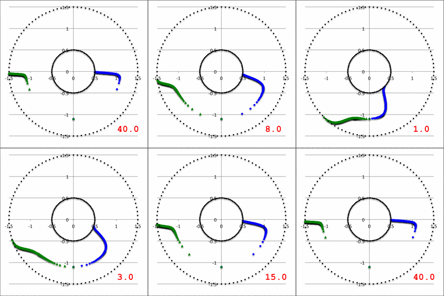
In the lefthand panel of Figure 4, the "constant phase loci" defined by this empirically constructed phase function has been mapped onto a polar-coordinate grid for ten different values of the leading coefficient in the range, <math>~1.0 \le \aleph \le 40.0</math>, as recorded in the bottom-right corner of the plot. The constant phase loci created by setting <math>~\aleph = 8.0</math> has been singled out and displayed in the middle panel of Figure 4, because it closely resembles the constant phase loci plot published by HI11a (reprinted here as the righthand panel of Figure 4 to facilitate comparison).

Figure 4
Constant Phase Loci Generated by Our Empirically Constructed Phase Function, <math>~\phi_1(\varpi)</math>		HI11's Published Constant Phase Loci
Ten Values of <math>~\aleph</math>	For <math>~\aleph = 8</math>	HI11's Published Constant Phase Loci

Discussion

Simpler Connection Between Radial and Phase Eigenfunctions

Define,

<math>~\Delta_\mathrm{inner}</math>	<math>~\equiv</math>	<math>~\biggl( \frac{\varpi - r_-}{r_\mathrm{mid}-r_-} \biggr)</math>	has range of	<math>~+0 ~~\rightarrow ~~ +1 \, ;</math>
<math>~\Delta_\mathrm{outer}</math>	<math>~\equiv</math>	<math>~\biggl( \frac{\varpi - r_+}{r_\mathrm{mid}-r_+} \biggr)</math>	has range of	<math>~+1 ~~\rightarrow ~~ +0 \, .</math>

We therefore also have, for the argument of ATANH,

<math>~1-2\Delta_\mathrm{inner}</math>	<math>~\equiv</math>	<math>~\biggl( \frac{\varpi - r_-}{r_\mathrm{mid}-r_-} \biggr)</math>	has range of	<math>~+1 ~~\rightarrow ~~ -1 \, ;</math>
<math>~1-2\Delta_\mathrm{outer}</math>	<math>~\equiv</math>	<math>~\biggl( \frac{\varpi - r_+}{r_\mathrm{mid}-r_+} \biggr)</math>	has range of	<math>~-1 ~~\rightarrow ~~ +1 \, .</math>

For the argument of <math>~D(\varpi)</math> function, we could therefore use,

<math>~1-\Delta_\mathrm{inner}</math>	<math>~\equiv</math>	<math>~\biggl( \frac{\varpi - r_-}{r_\mathrm{mid}-r_-} \biggr)</math>	has range of	<math>~+1 ~~\rightarrow ~~ 0 \, ;</math>
<math>~1-\Delta_\mathrm{outer}</math>	<math>~\equiv</math>	<math>~\biggl( \frac{\varpi - r_+}{r_\mathrm{mid}-r_+} \biggr)</math>	has range of	<math>~0 ~~\rightarrow ~~ +1 \, .</math>

User:Tohline/Appendix/Ramblings/Azimuthal Distortions

Contents