User:Tohline/Appendix/Ramblings/ForOuShangli
For Shangli Ou

|
|---|
| | Tiled Menu | Tables of Content | Banner Video | Tohline Home Page | |
EFE Diagram (Review)
|
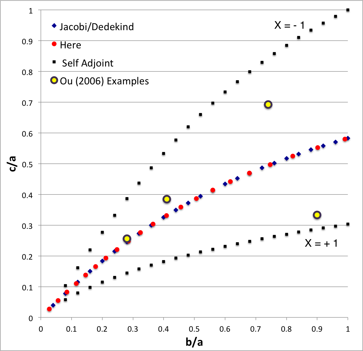
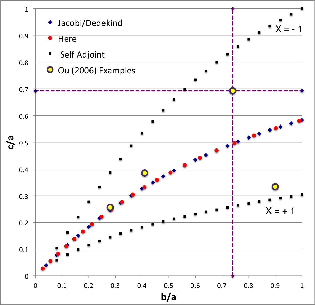
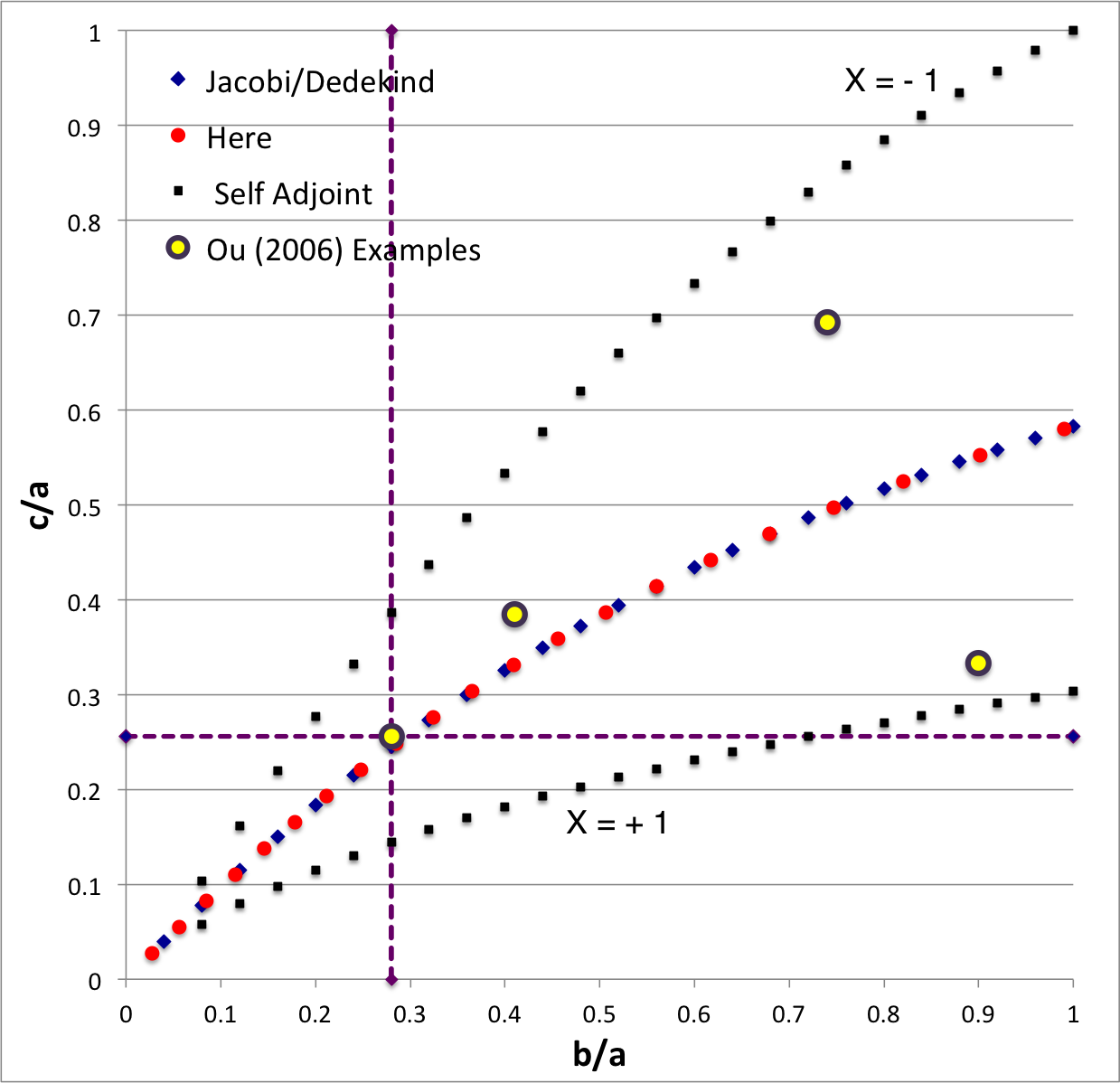
In the context of our broad discussion of ellipsoidal figures of equilibrium, the label "EFE Diagram" refers to a two-dimensional parameter space defined by the pair of axis ratios (b/a, c/a), usually covering the ranges, 0 ≤ b/a ≤ 1 and 0 ≤ c/a ≤ 1. The classic/original version of this diagram appears as Figure 2 on p. 902 of S. Chandrasekhar (1965, ApJ, vol. 142, pp. 890-921); a somewhat less cluttered version appears on p. 147 of Chandrasekhar's [EFE]. The version of the EFE Diagram shown here, on the left, highlights four model sequences, all of which also can be found in the original version:
Riemann S-type ellipsoids all lie between or on the two (self-adjoint) curves marked "X = -1" and "X = +1" in the EFE Diagram. The yellow circular markers in the diagram shown here, on the left, identify four Riemann S-type ellipsoids that were examined by Ou (2006) and that we have also chosen to use as examples. |
Example 3D Interactive Animations
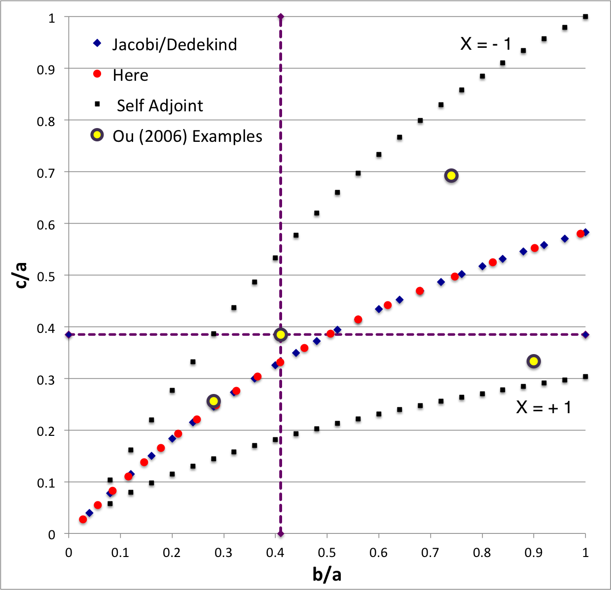
b41c385
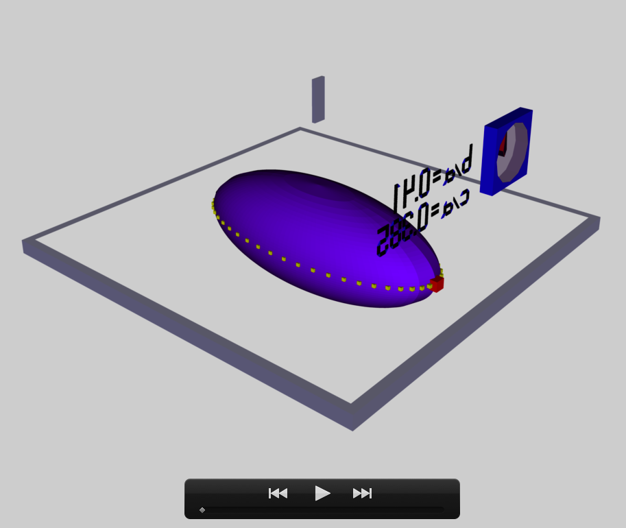
The model that we have chosen to use in our first successful construction of a COLLADA-based, 3D and interactive animation has the following properties; this model has been selected from Table 2 of our accompanying discussion of Riemann S-type ellipsoids:
|
|
<math>~\frac{b}{a} = 0.41</math> |
|
||||
|
<math>~\frac{c}{a} = 0.385</math> |
||||||
|
Direct |
|
Adjoint |
||||
|
<math>~\Omega_\mathrm{EFE} = 0.547874</math> |
<math>~\Omega_\mathrm{EFE} = - 0.079886</math> |
|||||
|
<math>~\lambda_\mathrm{EFE} = 0.079886</math> |
<math>~\lambda_\mathrm{EFE} = - 0.547874</math> |
|||||
|
<math>~f = - 0.415418</math> |
<math>~f = - 19.53923</math> |
|||||
The subscript "EFE" on Ω and λ means that the relevant frequency is given in units that have been adopted in [EFE], that is, in units of <math>~[\pi G\rho]^{1 / 2}</math>. In Figure 1a, the yellow circular marker, that has been placed where the pair of purple dashed lines cross, identifies the location of this model in the "c/a versus b/a" EFE Diagram that appears as Figure 2 on p. 902 of S. Chandrasekhar (1965); essentially the same diagram appears in §49 (p. 147) of [EFE].
In a separate chapter we have discussed various properties of uniformly rotating, Jacobi ellipsoids; they are equilibrium configurations that lie along the sequence that runs from "M2" (on the b/a = 1, Maclaurin sequence) to the origin of this diagram. Our chosen model lies off of — just above — the Jacobi-ellipsoid sequence, which means that it is not rotating as a solid body. Instead, as we focus first on the direct (as opposed to the adjoint) configuration, we appreciate that while the ellipsoid is spinning prograde (counter-clockwise) with a frequency given by |ΩEFE|, each Lagrangian fluid element inside as well as on the surface of the ellipsoid is traveling retrograde (clockwise) along an elliptical path with a frequency given by |λEFE|.
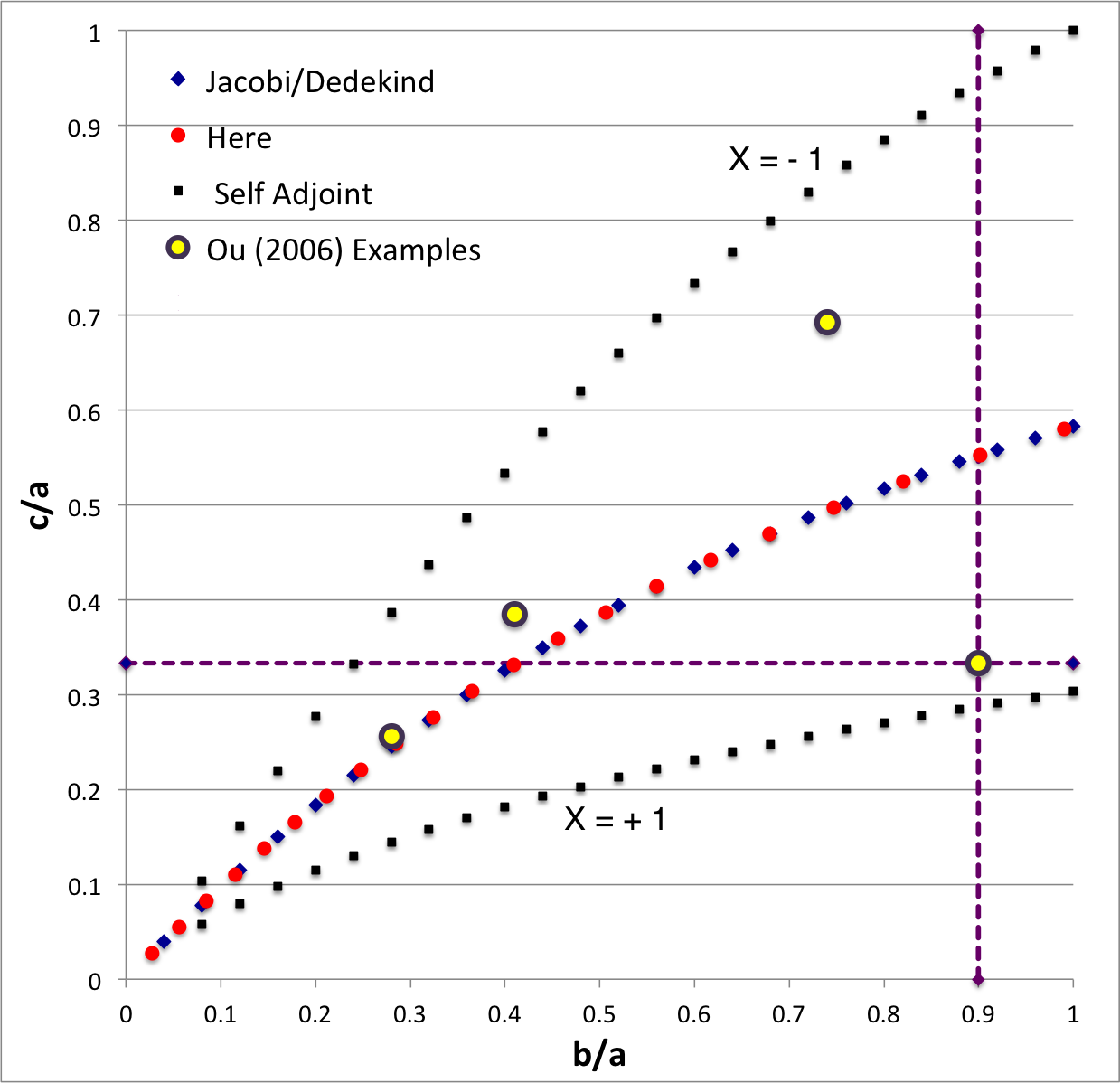
b90c333
The model that we have chosen to use in our second successful construction of a COLLADA-based, 3D and interactive animation has the following properties; this model has been selected from Table 2 of our accompanying discussion of Riemann S-type ellipsoids:
|
|
<math>~\frac{b}{a} = 0.90</math> |
|
||||
|
<math>~\frac{c}{a} = 0.333</math> |
||||||
|
Direct |
|
Adjoint |
||||
|
<math>~\Omega_\mathrm{EFE} = 0.447158</math> |
<math>~\Omega_\mathrm{EFE} = 0.221411</math> |
|||||
|
<math>~\lambda_\mathrm{EFE} = - 0.221411</math> |
<math>~\lambda_\mathrm{EFE} = - 0.447158 </math> |
|||||
|
<math>~f = + 0.995805</math> |
<math>~f = + 4.061607 </math> |
|||||
The subscript "EFE" on Ω and λ means that the relevant frequency is given in units that have been adopted in [EFE], that is, in units of <math>~[\pi G\rho]^{1 / 2}</math>. In Figure 1a, the yellow circular marker, that has been placed where the pair of purple dashed lines cross, identifies the location of this model in the "c/a versus b/a" EFE Diagram that appears as Figure 2 on p. 902 of S. Chandrasekhar (1965); essentially the same diagram appears in §49 (p. 147) of [EFE].
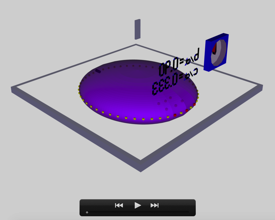
b74c692
The model that we have chosen to use in our second successful construction of a COLLADA-based, 3D and interactive animation has the following properties; this model has been selected from Table 2 of our accompanying discussion of Riemann S-type ellipsoids:
|
|
<math>~\frac{b}{a} = 0.74</math> |
|
||||
|
<math>~\frac{c}{a} = 0.692</math> |
||||||
|
Direct |
|
Adjoint |
||||
|
<math>~\Omega_\mathrm{EFE} = 0.638747</math> |
<math>~\Omega_\mathrm{EFE} = - 0.217773</math> |
|||||
|
<math>~\lambda_\mathrm{EFE} = 0.217773</math> |
<math>~\lambda_\mathrm{EFE} = - 0.638747 </math> |
|||||
|
<math>~f = - 0.713019</math> |
<math>~f = - 6.13413 </math> |
|||||
The subscript "EFE" on Ω and λ means that the relevant frequency is given in units that have been adopted in [EFE], that is, in units of <math>~[\pi G\rho]^{1 / 2}</math>. In Figure 1a, the yellow circular marker, that has been placed where the pair of purple dashed lines cross, identifies the location of this model in the "c/a versus b/a" EFE Diagram that appears as Figure 2 on p. 902 of S. Chandrasekhar (1965); essentially the same diagram appears in §49 (p. 147) of [EFE].
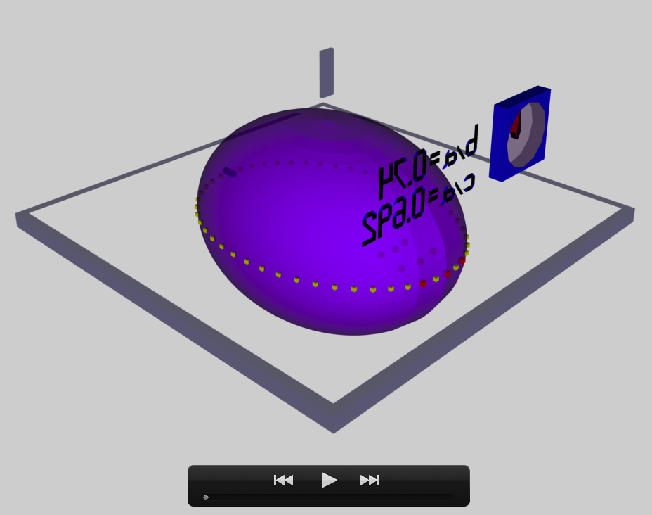
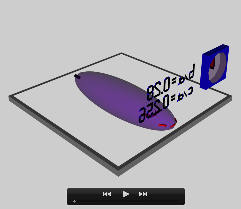
b28c256
The model that we have chosen to use in our second successful construction of a COLLADA-based, 3D and interactive animation has the following properties; this model has been selected from Table 2 of our accompanying discussion of Riemann S-type ellipsoids:
|
|
<math>~\frac{b}{a} = 0.28</math> |
|
||||
|
<math>~\frac{c}{a} = 0.256</math> |
||||||
|
Direct |
|
Adjoint |
||||
|
<math>~\Omega_\mathrm{EFE} = 0.456676</math> |
<math>~\Omega_\mathrm{EFE} = - 0.020692</math> |
|||||
|
<math>~\lambda_\mathrm{EFE} = 0.020692</math> |
<math>~\lambda_\mathrm{EFE} = - 0.456676</math> |
|||||
|
<math>~f = - 0.174510</math> |
<math>~f = - 85.0007</math> |
|||||
The subscript "EFE" on Ω and λ means that the relevant frequency is given in units that have been adopted in [EFE], that is, in units of <math>~[\pi G\rho]^{1 / 2}</math>. In Figure 1a, the yellow circular marker, that has been placed where the pair of purple dashed lines cross, identifies the location of this model in the "c/a versus b/a" EFE Diagram that appears as Figure 2 on p. 902 of S. Chandrasekhar (1965); essentially the same diagram appears in §49 (p. 147) of [EFE].

|
|---|
|
© 2014 - 2021 by Joel E. Tohline |
