Difference between revisions of "User:Tohline/SSC/Structure/BiPolytropes/Analytic5 1"
(→Instability: Rewrite key relations) |
(→Limiting Mass: Set group of defining equations into table format) |
||
| Line 1,046: | Line 1,046: | ||
We obtain, | We obtain, | ||
<div align="center"> | <div align="center"> | ||
<math> | <table border="0" cellpadding="5"> | ||
\eta_i = m_3 \biggl( \frac{\ell_i}{1 + \ell_i^2} \biggr) \, ; | |||
</ | <tr> | ||
<td align="right"> | |||
<math>\eta_i</math> | |||
</td> | |||
<td align="center"> | |||
<math>=</math> | |||
</td> | |||
<td align="left"> | |||
<math>m_3 \biggl( \frac{\ell_i}{1 + \ell_i^2} \biggr) \, ;</math> | |||
</td> | |||
</tr> | |||
<tr> | |||
<td align="right"> | |||
<math>\biggl( \frac{m_3}{\sqrt{1-m_3}} \biggr) \Lambda_i </math> | |||
</td> | |||
<td align="center"> | |||
<math>=</math> | |||
</td> | |||
<td align="left"> | |||
<math> | <math> | ||
U + \frac{1}{U} \, , | |||
</math> | </math> | ||
where, | where, | ||
| Line 1,058: | Line 1,077: | ||
U \equiv \sqrt{1-m_3}~\ell_i \, ; | U \equiv \sqrt{1-m_3}~\ell_i \, ; | ||
</math> | </math> | ||
</td> | |||
</tr> | |||
<math> | <tr> | ||
<td align="right"> | |||
</ | <math>A</math> | ||
</td> | |||
<td align="center"> | |||
<math>=</math> | |||
</td> | |||
<td align="left"> | |||
<math>\biggl[ \frac{1 + (1-m_3)^2 \ell_i^2}{1 + \ell_i^2} \biggr]^{1/2} \, ;</math> | |||
</td> | |||
</tr> | |||
<math> | <tr> | ||
\biggl( \frac{\pi}{2} \biggr)^{1/2} \frac{M_\mathrm{core}}{9} = \frac{\ell_i^3}{(1 + \ell_i^2)^{3/2}} \, ; | <td align="right"> | ||
</ | <math>\biggl( \frac{\pi}{2} \biggr)^{1/2} \frac{M_\mathrm{core}}{9}</math> | ||
</td> | |||
<td align="center"> | |||
<math>=</math> | |||
</td> | |||
<td align="left"> | |||
<math>\frac{\ell_i^3}{(1 + \ell_i^2)^{3/2}} \, ;</math> | |||
</td> | |||
</tr> | |||
<tr> | |||
<td align="right"> | |||
<math>\biggl( \frac{\pi}{2} \biggr)^{1/2} \frac{M_\mathrm{tot}}{9}</math> | |||
</td> | |||
<td align="center"> | |||
<math>=</math> | |||
</td> | |||
<td align="left"> | |||
<math> | <math> | ||
\frac{1}{m_3^2} \biggl[ 1 + (1-m_3)^2 \ell_i^2 \biggr]^{1/2} | |||
\biggl\{ \frac{\pi}{2} + m_3 \ell_i (1 + \ell_i^2)^{-1} + \tan^{-1}\biggl[ \frac{\sqrt{1-m_3}}{m_3} \biggl(U + \frac{1}{U} \biggr) \biggr] \biggr\} \, . | \biggl\{ \frac{\pi}{2} + m_3 \ell_i (1 + \ell_i^2)^{-1} + \tan^{-1}\biggl[ \frac{\sqrt{1-m_3}}{m_3} \biggl(U + \frac{1}{U} \biggr) \biggr] \biggr\} \, . | ||
</math> | </math> | ||
</td> | |||
</tr> | |||
</table> | |||
</div> | </div> | ||
Revision as of 02:45, 9 May 2013
BiPolytrope with <math>n_c = 5</math> and <math>n_e=1</math>

|
|---|
| | Tiled Menu | Tables of Content | Banner Video | Tohline Home Page | |
Here we construct a bipolytrope in which the core has an <math>n_c=5</math> polytropic index and the envelope has an <math>n_c=1</math> polytropic index. This system is particularly interesting because the entire structure can be described by closed-form, analytic expressions. As far as I have been able to determine, this analytic structural model has not previously been published in a refereed, archival journal (author: Joel E. Tohline, March 30, 2013). In deriving the properties of this model, we will follow the general solution steps for constructing a bipolytrope that we have outlined elsewhere.
Steps 2 & 3
Based on the discussion presented elsewhere of the structure of an isolated <math>n=5</math> polytrope, the core of this bipolytrope will have the following properties:
<math> \theta(\xi) = \biggl[ 1 + \frac{1}{3}\xi^2 \biggr]^{-1/2} ~~~~\Rightarrow ~~~~ \theta_i = \biggl[ 1 + \frac{1}{3}\xi_i^2 \biggr]^{-1/2} ; </math>
<math> \frac{d\theta}{d\xi} = - \frac{\xi}{3}\biggl[ 1 + \frac{1}{3}\xi^2 \biggr]^{-3/2} ~~~~\Rightarrow ~~~~ \biggl(\frac{d\theta}{d\xi}\biggr)_i = - \frac{\xi_i}{3}\biggl[ 1 + \frac{1}{3}\xi_i^2 \biggr]^{-3/2} \, . </math>
The first zero of the function <math>\theta(\xi)</math> and, hence, the surface of the corresponding isolated <math>n=5</math> polytrope is located at <math>\xi_s = \infty</math>. Hence, the interface between the core and the envelope can be positioned anywhere within the range, <math>0 < \xi_i < \infty</math>.
Step 4: Throughout the core (<math>0 \le \xi \le \xi_i</math>)
|
Specify: <math>K_c</math> and <math>\rho_0 ~\Rightarrow</math> |
|
|||
|
<math>\rho</math> |
<math>=</math> |
<math>\rho_0 \theta^{n_c}</math> |
<math>=</math> |
<math>\rho_0 \biggl( 1 + \frac{1}{3}\xi^2 \biggr)^{-5/2}</math> |
|
<math>P</math> |
<math>=</math> |
<math>K_c \rho_0^{1+1/n_c} \theta^{n_c + 1}</math> |
<math>=</math> |
<math>K_c \rho_0^{6/5} \biggl( 1 + \frac{1}{3}\xi^2 \biggr)^{-3}</math> |
|
<math>r</math> |
<math>=</math> |
<math>\biggl[ \frac{(n_c + 1)K_c}{4\pi G} \biggr]^{1/2} \rho_0^{(1-n_c)/(2n_c)} \xi</math> |
<math>=</math> |
<math>\biggl[ \frac{K_c}{G\rho_0^{4/5}} \biggr]^{1/2} \biggl(\frac{3}{2\pi}\biggr)^{1/2} \xi</math> |
|
<math>M_r</math> |
<math>=</math> |
<math>4\pi \biggl[ \frac{(n_c + 1)K_c}{4\pi G} \biggr]^{3/2} \rho_0^{(3-n_c)/(2n_c)} \biggl(-\xi^2 \frac{d\theta}{d\xi} \biggr)</math> |
<math>=</math> |
<math>\biggl[ \frac{K_c^3}{G^3 \rho_0^{2/5} } \biggr]^{1/2} \biggl( \frac{2\cdot 3}{\pi } \biggr)^{1/2} \biggl[ \xi^3 \biggl( 1 + \frac{1}{3}\xi^2 \biggr)^{-3/2} \biggr]</math> |
Step 5: Interface Conditions
|
|
Setting <math>n_c=5</math>, <math>n_e=1</math>, and <math>\phi_i = 1 ~~~~\Rightarrow</math> |
|||
|
<math>\frac{\rho_e}{\rho_0}</math> |
<math>=</math> |
<math>\biggl( \frac{\mu_e}{\mu_c} \biggr) \theta^{n_c}_i \phi_i^{-n_e}</math> |
<math>=</math> |
<math>\biggl( \frac{\mu_e}{\mu_c} \biggr) \theta^{5}_i </math> |
|
<math>\biggl( \frac{K_e}{K_c} \biggr) </math> |
<math>=</math> |
<math>\rho_0^{1/n_c - 1/n_e}\biggl( \frac{\mu_e}{\mu_c} \biggr)^{-(1+1/n_e)} \theta^{1 - n_c/n_e}_i</math> |
<math>=</math> |
<math>\rho_0^{-4/5}\biggl( \frac{\mu_e}{\mu_c} \biggr)^{-2} \theta^{-4}_i</math> |
|
<math>\frac{\eta_i}{\xi_i}</math> |
<math>=</math> |
<math>\biggl[ \frac{n_c + 1}{n_e+1} \biggr]^{1/2} \biggl( \frac{\mu_e}{\mu_c}\biggr) \theta_i^{(n_c-1)/2} \phi_i^{(1-n_e)/2}</math> |
<math>=</math> |
<math>3^{1/2} \biggl( \frac{\mu_e}{\mu_c}\biggr) \theta_i^{2}</math> |
|
<math>\biggl( \frac{d\phi}{d\eta} \biggr)_i</math> |
<math>=</math> |
<math>\biggl[ \frac{n_c + 1}{n_e + 1} \biggr]^{1/2} \theta_i^{- (n_c + 1)/2} \phi_i^{(n_e+1)/2} \biggl( \frac{d\theta}{d\xi} \biggr)_i</math> |
<math>=</math> |
<math>3^{1/2} \theta_i^{- 3} \biggl( \frac{d\theta}{d\xi} \biggr)_i</math> |
Step 6: Envelope Solution
Adopting equation (8) of Beech (1988), the most general solution to the <math>n=1</math> Lane-Emden equation can be written in the form,
<math> \phi = A \biggl[ \frac{\sin(\eta - B)}{\eta} \biggr] \, , </math>
where <math>A</math> and <math>B</math> are constants. The first derivative of this function is,
<math> \frac{d\phi}{d\eta} = \frac{A}{\eta^2} \biggl[ \eta\cos(\eta-B) - \sin(\eta-B) \biggr] \, . </math>
From Step 5, above, we know the value of the function, <math>\phi</math> and its first derivative at the interface; specifically,
<math> \phi_i = 1~~~~\mathrm{and} ~~~~\biggl( \frac{d\phi}{d\eta}\biggr)_i =3^{1/2} \theta_i^{- 3} \biggl( \frac{d\theta}{d\xi} \biggr)_i~~~~ \mathrm{at}~~~~\eta_i =3^{1/2} \xi_i \biggl( \frac{\mu_e}{\mu_c}\biggr) \theta_i^{2}</math>
From this information we can determine the constants <math>A</math> and <math>B</math>; specifically,
<math> \eta_i - B = \tan^{-1}(\Lambda_i^{-1}) = \frac{\pi}{2}- \tan^{-1}(\Lambda_i) \, , </math>
<math> A = \frac{\phi_i \eta_i}{\sin(\eta_i - B)} = \phi_i \eta_i (1 + \Lambda_i^2)^{1/2} \, , </math>
where,
<math> \Lambda_i = \frac{1}{\eta_i} + \frac{1}{\phi_i} \biggl(\frac{d\phi}{d\eta}\biggr)_i \, . </math>
Step 7
The surface will be defined by the location, <math>\eta_s</math>, at which the function <math>\phi(\eta)</math> first goes to zero, that is,
<math> \eta_s = \pi + B = \frac{\pi}{2} + \eta_i + \tan^{-1}(\Lambda_i) \, . </math>
Step 8: Throughout the envelope (<math>\eta_i \le \eta \le \eta_s</math>)
|
|
Knowing: <math>K_e/K_c</math> and <math>\rho_e/\rho_0</math> from Step 5 <math>\Rightarrow</math> |
|||||
|
<math>\rho</math> |
<math>=</math> |
<math>\rho_e \phi^{n_e}</math> |
<math>=</math> |
<math>\rho_0 \biggl(\frac{\rho_e}{\rho_0}\biggr) \phi</math> |
<math>=</math> |
<math>\rho_0 \biggl( \frac{\mu_e}{\mu_c} \biggr) \theta^{5}_i \phi</math> |
|
<math>P</math> |
<math>=</math> |
<math>K_e \rho_e^{1+1/n_e} \phi^{n_e + 1}</math> |
<math>=</math> |
<math>K_c \rho_0^{6/5} \biggl(\frac{K_e \rho_0^{4/5}}{K_c}\biggr) \biggl(\frac{\rho_e}{\rho_0}\biggr)^{2} \phi^{2}</math> |
<math>=</math> |
<math>K_c \rho_0^{6/5} \theta^{6}_i \phi^{2}</math> |
|
<math>r</math> |
<math>=</math> |
<math>\biggl[ \frac{(n_e + 1)K_e}{4\pi G} \biggr]^{1/2} \rho_e^{(1-n_e)/(2n_e)} \eta</math> |
<math>=</math> |
<math>\biggl[ \frac{K_c}{G \rho_0^{4/5}} \biggr]^{1/2} \biggl( \frac{K_e \rho_0^{4/5}}{K_c} \biggr)^{1/2} (2\pi)^{-1/2}\eta</math> |
<math>=</math> |
<math>\biggl[ \frac{K_c}{G \rho_0^{4/5}} \biggr]^{1/2} \biggl( \frac{\mu_e}{\mu_c} \biggr)^{-1} \theta^{-2}_i (2\pi)^{-1/2}\eta</math> |
|
<math>M_r</math> |
<math>=</math> |
<math>4\pi \biggl[ \frac{(n_e + 1)K_e}{4\pi G} \biggr]^{3/2} \rho_e^{(3-n_e)/(2n_e)} \biggl(-\eta^2 \frac{d\phi}{d\eta} \biggr)</math> |
<math>=</math> |
<math>\biggl[ \frac{K_c^3}{G^3 \rho_0^{2/5}} \biggr]^{1/2} \biggl( \frac{K_e \rho_0^{4/5}}{K_c} \biggr)^{3/2} \biggl(\frac{\rho_e}{\rho_0}\biggr) \biggl( \frac{2}{\pi} \biggr)^{1/2} \biggl(-\eta^2 \frac{d\phi}{d\eta} \biggr)</math> |
<math>=</math> |
<math>\biggl[ \frac{K_c^3}{G^3 \rho_0^{2/5}} \biggr]^{1/2} \biggl( \frac{\mu_e}{\mu_c} \biggr)^{-2} \theta^{-1}_i \biggl( \frac{2}{\pi} \biggr)^{1/2} \biggl(-\eta^2 \frac{d\phi}{d\eta} \biggr)</math> |
Examples
Normalization
The dimensionless variables used in Tables 1 & 2 are defined as follows:
|
<math>\rho^*</math> |
<math>\equiv</math> |
<math>\frac{\rho}{\rho_0}</math> |
; |
<math>r^*</math> |
<math>\equiv</math> |
<math>\frac{r}{[K_c^{1/2}/(G^{1/2}\rho_0^{2/5})]}</math> |
|
<math>P^*</math> |
<math>\equiv</math> |
<math>\frac{P}{K_c\rho_0^{6/5}}</math> |
; |
<math>M_r^*</math> |
<math>\equiv</math> |
<math>\frac{M_r}{[K_c^{3/2}/(G^{3/2}\rho_0^{1/5})]}</math> |
|
<math>H^*</math> |
<math>\equiv</math> |
<math>\frac{H}{K_c\rho_0^{1/5}}</math> |
. |
|
||
Parameter Values
The <math>2^\mathrm{nd}</math> column of Table 1 catalogues the analytic expressions that define various parameters and physical properties (as identified, respectively, in column 1) of the <math>n_c=5</math>, <math>n_e=1</math> bipolytrope. We have evaluated these expressions for various choices of the dimensionless interface radius, <math>\xi_i</math>, and have tabulated the results in the last few columns of the table. The tabulated values have been derived assuming <math>\mu_e/\mu_c = 1</math>, that is, assuming that the core and the envelope have the same mean molecular weights.
Table 1: Properties of <math>n_c=5</math>, <math>n_e=1</math>, BiPolytrope Having Various Interface Locations, <math>\xi_i</math>
File:BiPolytropeParametersV01.xml
|
Parameter |
<math>\xi_i</math> |
0.5 |
1.0 |
3.0 |
|
<math>\theta_i</math> |
<math>\biggl( 1+\frac{1}{3}\xi_i^2 \biggr)^{-1/2}</math> |
0.96077 |
0.86603 |
0.50000 |
|
<math>-\biggl(\frac{d\theta_i}{d\xi}\biggr)_i</math> |
<math>\frac{1}{3} \xi_i \biggl( 1+\frac{1}{3}\xi_i^2 \biggr)^{-3/2}</math> |
0.14781 |
0.21651 |
0.12500 |
|
<math>r^*_\mathrm{core} \equiv r^*_i</math> |
<math>\biggl( \frac{3}{2\pi} \biggr)^{1/2} \xi_i</math> |
0.34549 |
0.69099 |
2.07297 |
|
<math>\rho^*_i \biggr|_c = \biggl( \frac{\mu_e}{\mu_c} \biggr)^{-1} \rho^*_i \biggr|_e</math> |
<math>\biggl( 1+\frac{1}{3}\xi_i^2 \biggr)^{-5/2}</math> |
0.81864 |
0.48714 |
0.03125 |
|
<math>P^*_i</math> |
<math>\biggl( 1+\frac{1}{3}\xi_i^2 \biggr)^{-3}</math> |
0.78653 |
0.42188 |
0.01563 |
|
<math>H^*_i \biggr|_c = \frac{n_c+1}{n_e+1} \biggl( \frac{\mu_e}{\mu_c} \biggr) H^*_i \biggr|_e</math> |
<math>6 \biggl( 1+\frac{1}{3}\xi_i^2 \biggr)^{-1/2}</math> |
5.76461 |
5.19615 |
3.00000 |
|
<math>M^*_\mathrm{core}</math> |
<math>\biggl( \frac{6}{\pi}\biggr)^{1/2} (\xi_i \theta_i)^3</math> |
0.15320 |
0.89762 |
4.66417 |
|
<math>\biggl( \frac{\mu_e}{\mu_c} \biggr)^{-1}\eta_i</math> |
<math>\sqrt{3} ~\theta_i^2 \xi_i</math> |
0.79941 |
1.29904 |
1.29904 |
|
<math>-\biggl( \frac{d\phi}{d\eta} \biggr)_i</math> |
<math>\sqrt{3} ~\theta_i^{-3} \biggl( - \frac{d\theta}{d\xi} \biggr)_i = \frac{\xi_i}{\sqrt{3}}</math> |
0.28868 |
0.57735 |
1.73205 |
|
<math>\Lambda_i</math> |
<math>\frac{1}{\eta_i} + \biggl( \frac{d\phi}{d\eta} \biggr)_i</math> |
0.96225 |
0.19245 |
-0.96225 |
|
<math>A</math> |
<math>\eta_i (1 + \Lambda_i^2)^{1/2}</math> |
1.10940 |
1.32288 |
1.80278 |
|
<math>B</math> |
<math>\eta_i - \frac{\pi}{2} + \tan^{-1}( \Lambda_i)</math> |
- 0.00523 |
-0.08163 |
-1.03792 |
|
<math>\eta_s</math> |
<math>\pi + B</math> |
3.13637 |
3.05996 |
2.10367 |
|
<math>- \biggl( \frac{d\phi}{d\eta} \biggr)_s</math> |
<math>\frac{A}{\eta_s}</math> |
0.35372 |
0.43232 |
0.85697 |
|
<math>\biggl( \frac{\mu_e}{\mu_c} \biggr) \cdot \biggl[ R^* \equiv r^*_s \biggr]</math> |
<math>\frac{\eta_s}{\sqrt{2\pi} ~\theta_i^2}</math> |
1.35550 |
1.62766 |
3.35697 |
|
<math>\biggl( \frac{\mu_e}{\mu_c} \biggr)^2 M^*_\mathrm{tot}</math> |
<math>\biggl(\frac{2}{\pi}\biggr)^{1/2} \theta_i^{-1} \biggl( -\eta^2 \frac{d\phi}{d\eta} \biggr)_s = \biggl(\frac{2}{\pi}\biggr)^{1/2} \frac{A\eta_s}{\theta_i}</math> |
2.88959 |
3.72945 |
6.05187 |
|
<math>\biggl(\frac{\mu_e}{\mu_c}\biggr)^{-2} \cdot \biggl[ \nu \equiv \frac{M_\mathrm{core}}{M_\mathrm{tot}} \biggr]</math> |
<math>\sqrt{3} ~\biggl( \frac{\xi_i^3 \theta_i^4}{A\eta_s} \biggr)</math> |
0.05302 |
0.24068 |
0.77070 |
|
<math>\biggl(\frac{\mu_e}{\mu_c}\biggr)^{-1} \cdot \biggl[ q \equiv \frac{r_\mathrm{core}}{R} \biggr]</math> |
<math>\sqrt{3}~\biggl[\frac{\xi_i \theta_i^2}{\eta_s}\biggr]</math> |
0.25488 |
0.42453 |
0.61751 |
Profile
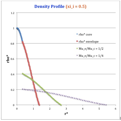
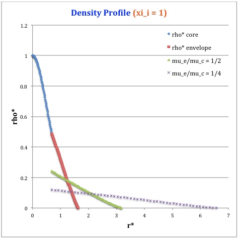
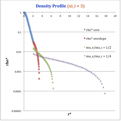
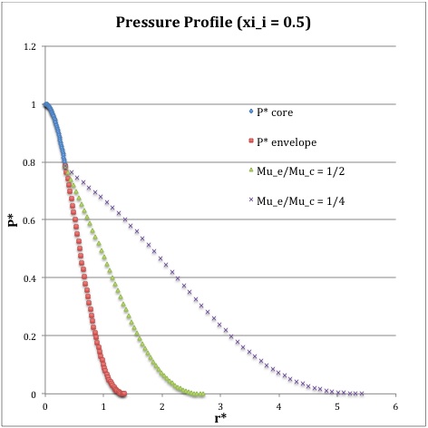
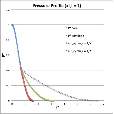
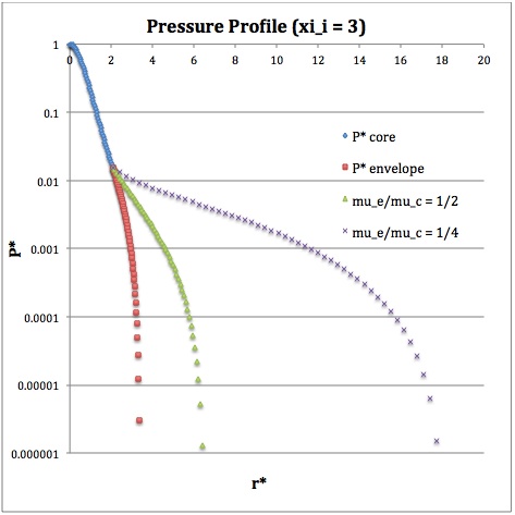
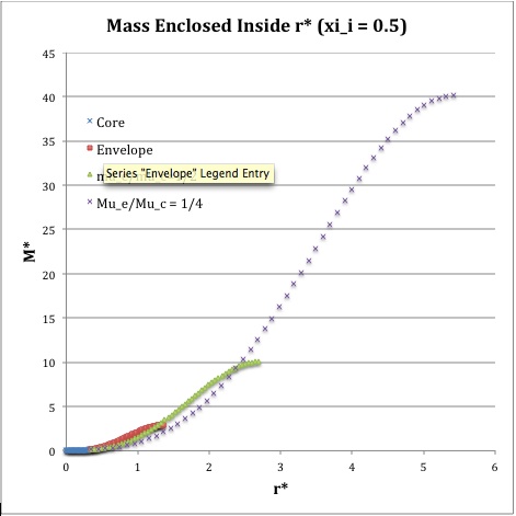
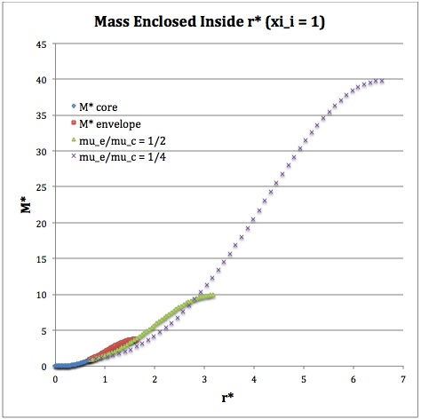
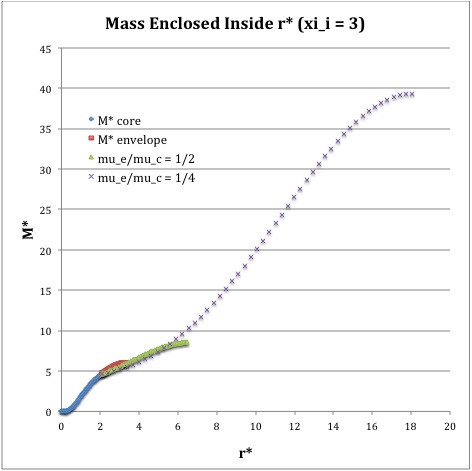
Once the values of the key set of parameters have been determined as illustrated in Table 1, the radial profile of various physical variables can be determined throughout the bipolytrope as detailed in step #4 and step #8, above. Table 2 summarizes the mathematical expressions that define the profile throughout the core (column 2) and throughout the envelope (column 3) of the normalized mass density, <math>\rho^*(r^*)</math>, the normalized gas pressure, <math>P^*(r^*)</math>, and the normalized mass interior to <math>r^*</math>, <math>M_r^*(r^*)</math>. For all profiles, the relevant normalized radial coordinate is <math>r^*</math>, as defined in the <math>2^\mathrm{nd}</math> row of Table 2. Graphical illustrations of these resulting profiles can be viewed by clicking on the thumbnail images posted in the last few columns of Table 2.
Table 2: Radial Profile of Various Physical Variables
|
Variable |
Throughout the Core |
Throughout the Envelope† |
Plotted Profiles |
||
|
<math>\xi_i = 0.5</math> |
<math>\xi_i = 1.0</math> |
<math>\xi_i = 3.0</math> |
|||
|
<math>r^*</math> |
<math>\biggl( \frac{3}{2\pi} \biggr)^{1/2} \xi</math> |
<math>\biggl( \frac{\mu_e}{\mu_c} \biggr)^{-1} \theta^{-2}_i (2\pi)^{-1/2}\eta</math> |
|
||
|
<math>\rho^*</math> |
<math>\biggl( 1 + \frac{1}{3}\xi^2 \biggr)^{-5/2}</math> |
<math>\biggl( \frac{\mu_e}{\mu_c} \biggr) \theta^{5}_i \phi(\eta)</math> |
|||
|
<math>P^*</math> |
<math>\biggl( 1 + \frac{1}{3}\xi^2 \biggr)^{-3}</math> |
<math>\theta^{6}_i [\phi(\eta)]^{2}</math> |
|||
|
<math>M_r^*</math> |
<math>\biggl( \frac{2\cdot 3}{\pi } \biggr)^{1/2} \biggl[ \xi^3 \biggl( 1 + \frac{1}{3}\xi^2 \biggr)^{-3/2} \biggr]</math> |
<math>\biggl( \frac{\mu_e}{\mu_c} \biggr)^{-2} \theta^{-1}_i \biggl( \frac{2}{\pi} \biggr)^{1/2} \biggl(-\eta^2 \frac{d\phi}{d\eta} \biggr)</math> |
|||
|
†In order to obtain the various envelope profiles, it is necessary to evaluate <math>\phi(\eta)</math> and its first derivative using the information presented in Step 6, above. |
|||||
[As of 28 April 2013] For the interface locations <math>\xi_i = 0.5, ~1.0,~\mathrm{and}~3.0</math>, Table 2 provides profiles for three values of the molecular weight ratio: <math>\mu_e/\mu_c = 1.0, ~1/2,~\mathrm{and}~1/4</math>. In all nine graphs, blue diamonds trace the structure of the <math>n_c=5</math> core; the core extends to a radius, <math>r^*_\mathrm{core}</math>, that is independent of molecular weight ratio but varies in direct proportion to the choice of <math>\xi_i</math>. Specifically, as tabulated in the fourth row of Table 1, <math>r^*_\mathrm{core} = 0.34549, ~0.69099, ~\mathrm{and} ~2.07297</math> for, respectively, <math>\xi_i = 0.5,~1,~\mathrm{and}~3</math>. Notice that, while the pressure profile and mass profile are continuous at the interface for all choices of the molecular weight ratio, the density profile exhibits a discontinuous jump that is in direct proportion to the chosen value of <math>\mu_e/\mu_c</math>.
Throughout the <math>n_e = 1</math> envelope, the profile of all physical variables varies with the choice of the molecular weight ratio. In the Table 2 graphs, red squares trace the envelope profile for <math>\mu_e/\mu_c = 1.0</math>; green triangles trace the envelope profile for <math>\mu_e/\mu_c = 1/2</math>; and purple crosses trace the envelope profile for <math>\mu_e/\mu_c = 1/4</math>. The surface of the bipolytropic configuration is defined by the (normalized) radius, <math>R^*</math>, at which the envelope density and pressure drop to zero; the values tabulated in row 16 of Table 1 — <math>1.35550, ~1.62766, ~\mathrm{and} ~3.35697</math> for, respectively, <math>\xi_i = 0.5,~1,~\mathrm{and}~3</math> — correspond to a molecular weight ratio of unity and, hence also, to the envelope profiles traced by red squares in the Table 2 graphs. As the molecular weight ratio is decreased from unity to <math>1/2</math> and, then, <math>1/4</math> for a given choice of <math>\xi_i</math>, the (normalized) radius of the bipolytrope increases roughly in inverse proportion to <math>\mu_e/\mu_c</math> as suggested by the formula for <math>R^*</math> shown in Table 1. This proportional relation is not exact, however, because the parameter <math>\eta_s</math>, which also appears in the formula for <math>R^*</math>, contains an implicit dependence on the chosen value of the molecular weight ratio through the parameter <math>\eta_i</math>.
For a given choice of the interface parameter, <math>\xi_i</math>, the (normalized) mass that is contained in the core is independent of the choice of the molecular weight ratio. However, the (normalized) total mass, <math>M_\mathrm{tot}^*</math>, varies significantly with the choice of <math>\mu_e/\mu_c</math>; as suggested by the expression provided in row 17 of Table 1, the variation is in rough proportion to <math>(\mu_e/\mu_c)^{-2}</math> but, as with <math>R^*</math>, this proportional relation is not exact because the parameters <math>\eta_s</math> and <math>A</math> which also appear in the formula for <math>M_\mathrm{tot}^*</math> harbor an implicit dependence on the molecular weight ratio.
Model Sequences
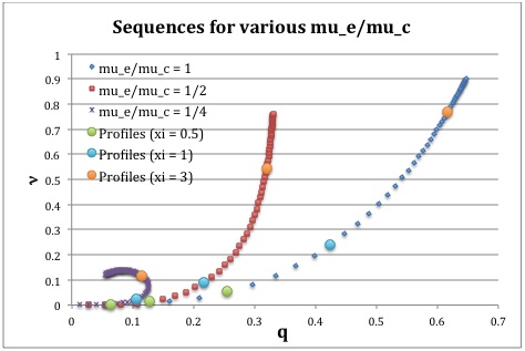
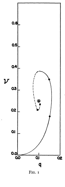
For a given choice of <math>\mu_e/\mu_c</math> a physically relevant sequence of models can be constructed by steadily increasing the value of <math>\xi_i</math> from zero to infinity — or at least to some value, <math>\xi_i \gg 1</math>. Figure 1 shows how the fractional core mass, <math>\nu \equiv M_\mathrm{core}/M_\mathrm{tot}</math>, varies with the fractional core radius, <math>q \equiv r_\mathrm{core}/R</math>, along sequences for which <math>\mu_e/\mu_c = 1</math> (blue diamonds), <math>\mu_e/\mu_c = 1/2</math> (red squares), and <math>\mu_e/\mu_c = 1/4</math> (purple crosses). On each of the displayed sequences, the point marked by a solid light-green circle identifies the model for which <math>\xi_i = 0.5</math>; the solid light-blue circle identifies the model for which <math>\xi_i = 1</math>; and the solid orange circle identifies the model for which <math>\xi_i = 3</math>. The images linked to Table 2 provide plots of the density, pressure and mass profiles for these nine models.
The natural expectation is that an increase in <math>\xi_i</math> along a given sequence will correspond to an increase in the relative size — both the radius and the mass — of the core. This expectation is realized along the sequences marked by blue symbols (<math>\mu_e/\mu_c = 1</math>) and by red symbols (<math>\mu_e/\mu_c = 1/2</math>). But the behavior is different along the <math>\mu_e/\mu_c = 1/4</math> model sequence. For sufficiently large <math>\xi_i</math>, the relative radius of the core begins to decrease; then, as <math>\xi_i</math> is pushed to even larger values, eventually the relative core mass begins to decrease.
|
Figure 1: Fractional mass versus fractional radius along several equilibrium sequences |
|
|
Caption: Analytically determined plot of fractional core mass (<math>\nu</math>) versus fractional core radius (<math>q</math>) for <math>n_c=5</math>, <math>n_e=1</math> bipolytrope model sequences having <math>\mu_e/\mu_c = 1</math> (blue diamonds), <math>\mu_e/\mu_c = 1/2</math> (red squares), and <math>\mu_e/\mu_c = 1/4</math> (purple crosses). The points marked by solid-colored circles correspond to models for which radial profiles of various physical variables are provided in Table 2. Along each of the three separate model sequences, the light green point corresponds to the model whose interface parameter <math>\xi_i = 0.5</math>; the light blue point corresponds to the model with <math>\xi_i = 1</math>; and the orange point corresponds to the model with <math>\xi_i = 3</math>. |
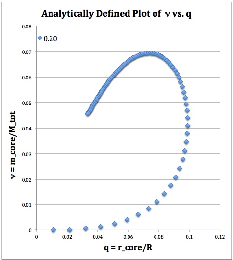
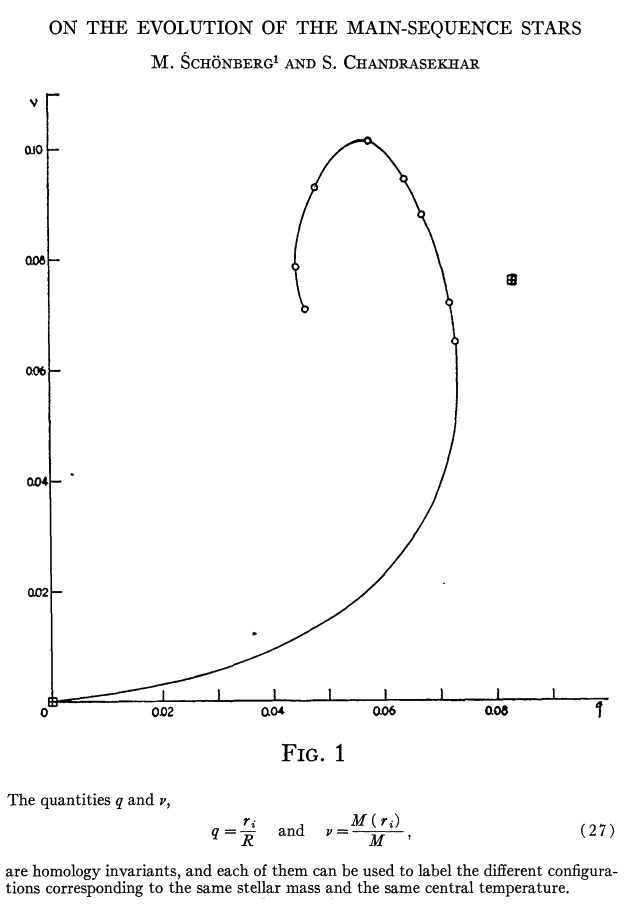
The variation of <math>\nu</math> with <math>q</math> for a fourth analytically determined model sequence — one for which <math>\mu_e/\mu_c = 1/5</math> — is mapped out by a string of blue diamond symbols in the left-hand side of Figure 2. It behaves in an analogous fashion to the <math>\mu_e/\mu_c = 1/4</math> sequence (marked by purple crosses) displayed in Figure 1. It also quantitatively, as well as qualitatively, resembles the sequence that was numerically constructed by Schönberg & Chandrasekhar (1942) for models with an isothermal core (<math>n_c = \infty</math>) and an <math>n_e=3/2</math> envelope; Fig. 1 from their paper has been reproduced here on the right-hand side of Figure 2.
|
Figure 2: Relationship to Schönberg-Chandrasekhar Mass Limit |
||
|
Analytic BiPolytrope with <math>n_c=5</math>, <math>n_e = 1</math>, and <math>\mu_e/\mu_c = 1/5</math> |
Edited excerpt from Schönberg & Chandrasekhar (1942) |
Figure from Henrich & Chandraskhar (1941) |
|
(Above) Plot of fractional core mass (<math>\nu</math>) versus fractional core radius (<math>q</math>) for the analytic bipolytrope having <math>\mu_e/\mu_c = 1/5</math>. The behavior of this analytically defined model sequence resembles the behavior of the numerically constructed isothermal core models presented by (center) Schönberg & Chandrasekhar (1942) and by (far right) Henrich & Chandraskhar (1941). |
||
Instability
Limiting Mass
As early as 1941, Chandraskhar and his collaborators realized that the shape of the model sequence in a <math>\nu</math> versus <math>q</math> diagram, as displayed in Figure 2 above, implies that equilibrium structures can exist only if the fractional core mass lies below some limiting value. This realization is documented, for example, by the following excerpt from §5 of Henrich & Chandraskhar (1941).
|
Text excerpt from Henrich & Chandraskhar (1941) |
|
Given that our bipolytropic sequence has been defined analytically, it may be possible to analytically determine the limiting core mass of our model. In order to accomplish this, we need to identify the point along the sequence — in particular, the value of the dimensionless interface location — at which <math>d\nu/dq = 0</math> or, equivalently, <math>d\nu/d\xi_i = 0</math>.
Before carrying out the desired differentiations, we will find it useful to rewrite the relevant expressions in terms of the parameters,
<math> \ell_i \equiv \frac{\xi_i}{\sqrt{3}} \, ; </math> and <math> m_3 \equiv 3 \biggl( \frac{\mu_e}{\mu_c} \biggr) \, . </math>
We obtain,
|
<math>\eta_i</math> |
<math>=</math> |
<math>m_3 \biggl( \frac{\ell_i}{1 + \ell_i^2} \biggr) \, ;</math> |
|
<math>\biggl( \frac{m_3}{\sqrt{1-m_3}} \biggr) \Lambda_i </math> |
<math>=</math> |
<math> U + \frac{1}{U} \, , </math> where, <math> U \equiv \sqrt{1-m_3}~\ell_i \, ; </math> |
|
<math>A</math> |
<math>=</math> |
<math>\biggl[ \frac{1 + (1-m_3)^2 \ell_i^2}{1 + \ell_i^2} \biggr]^{1/2} \, ;</math> |
|
<math>\biggl( \frac{\pi}{2} \biggr)^{1/2} \frac{M_\mathrm{core}}{9}</math> |
<math>=</math> |
<math>\frac{\ell_i^3}{(1 + \ell_i^2)^{3/2}} \, ;</math> |
|
<math>\biggl( \frac{\pi}{2} \biggr)^{1/2} \frac{M_\mathrm{tot}}{9}</math> |
<math>=</math> |
<math> \frac{1}{m_3^2} \biggl[ 1 + (1-m_3)^2 \ell_i^2 \biggr]^{1/2} \biggl\{ \frac{\pi}{2} + m_3 \ell_i (1 + \ell_i^2)^{-1} + \tan^{-1}\biggl[ \frac{\sqrt{1-m_3}}{m_3} \biggl(U + \frac{1}{U} \biggr) \biggr] \biggr\} \, . </math> |
Related Discussions

|
|---|
|
© 2014 - 2021 by Joel E. Tohline |
