User:Tohline/SSC/Structure/BiPolytropes

BiPolytropes

This discussion of bipolytropes is built upon the early ideas and mathematical foundation laid out by Milne (1930), Cowling (1931), Schönberg & Chandrasekhar (1942) and, especially, §28 (pp. 171-174) of [C67].

Background

While polytropic spheres can give us useful general insight into the internal structure of stars, they do not faithfully represent the detailed structure of most stars, in part, because the equation of state that is most relevant to the densest regions of a star usually is different from the equation of state that is relevant to the star's envelope. As is highlighted in the following excerpt from Cowling (1931), Milne (1930) was among the first to suggest that more realism could be achieved by constructing what is now commonly referred to as a bipolytrope: a composite model in which the envelope, obeying one equation of state — described by polytropic index <math>n_e</math> — is fitted to a core obeying a different equation of state — described by polytropic index <math>n_c</math>.

Excerpt from the introductory paragraphs of Cowling (1931)

Milne (1930) envisioned that the temperature, <math>T</math>, and pressure, <math>P</math>, should be "continuous across the surface of fit." Given that <math>P</math> and <math>T</math> are continuous, he envisioned that the gas density, <math>\rho</math>, should be continuous across the surface of fit as well. Schönberg & Chandrasekhar (1942) later pointed out — see the following journal article excerpt — that, if the core and envelope have different molecular weights, it is the ratio <math>\rho/\mu</math> that should be continuous across the interface. A discontinuous jump in <math>\mu</math> at the interface — for example, switching from a pure helium core to an envelope whose dominant element is hydrogen — will therefore lead to a discontinuous jump (of reciprocal value) in the density at the interface.

Excerpt from §2 of Schönberg & Chandrasekhar (1942)

<imagemap> Image:SchonbergChandra1942.jpg|600px|References rect 0 480 210 580 User:Tohline/PGE rect 260 480 850 580 User:Tohline/Appendix/References#C67 desc none </imagemap>

Schönberg & Chandrasekhar (1942) furthermore pointed out — again, see the above excerpt — that, when constructing a bipolytropic model, the mathematical function that specifies the mass enclosed inside a spherical radius <math>r</math> for the core, <math>M(r)|_\mathrm{c}</math>, must give the same value as the mathematical function that specifies the mass enclosed inside a spherical radius <math>r</math> for the envelope, <math>M(r)|_\mathrm{e}</math> at the radial location of the interface, <math>r_i</math>.

Setup

Isothermal <math>(n = \infty)</math>	<math>n = n_1</math>	<math>n = n_2</math>
<math> \frac{1}{\chi^2} \frac{d}{d\chi} \biggl( \chi^2 \frac{d\psi}{d\chi} \biggr) = e^{-\psi} </math> sol'n: <math> \psi(\chi) </math>	<math> \frac{1}{\xi^2} \frac{d}{d\xi} \biggl( \xi^2 \frac{d\theta}{d\xi} \biggr) = \theta^{n_1} </math> sol'n: <math> \theta(\xi) </math>	<math> \frac{1}{\eta^2} \frac{d}{d\eta} \biggl( \eta^2 \frac{d\phi}{d\eta} \biggr) = \phi^{n_2} </math> sol'n: <math> \phi(\eta) </math>
Specify: <math>c_s^2</math> and <math>\rho_0 ~\Rightarrow</math> <math>\rho</math> <math>=</math> <math>\rho_0 e^{-\psi}</math> <math>P</math> <math>=</math> <math>c_s^2 \rho_0 e^{-\psi}</math> <math>r</math> <math>=</math> <math>\biggl[ \frac{c_s^2}{4\pi G\rho_0} \biggr]^{1/2} \chi</math> <math>M_r</math> <math>=</math> <math>\biggl[ \frac{c_s^6}{4\pi G^3\rho_0} \biggr]^{1/2} \biggl( \chi^2 \frac{d\psi}{d\chi} \biggr)</math>	Specify: <math>K_1</math> and <math>\lambda_1 ~\Rightarrow</math> <math>\rho</math> <math>=</math> <math>\lambda_1 \theta^{n_1}</math> <math>P</math> <math>=</math> <math>K_1 \lambda_1^{1+1/n_1} \theta^{n_1 + 1}</math> <math>r</math> <math>=</math> <math>\biggl[ \frac{(n_1 + 1)K_1}{4\pi G} \biggr]^{1/2} \lambda_1^{(1-n_1)/(2n_1)} \xi</math> <math>M_r</math> <math>=</math> <math>4\pi \biggl[ \frac{(n_1 + 1)K_1}{4\pi G} \biggr]^{3/2} \lambda_1^{(3-n_1)/(2n_1)} \biggl( -\xi^2 \frac{d\theta}{d\xi} \biggr)</math>

Old Material

As has been derived and discussed elsewhere, an isolated isothermal sphere has a density profile that extends to infinity and, correspondingly, an unbounded total mass. In an astrophysical context, neither of these properties is desirable. A more realistic isothermal configuration can be constructed by embedding the structure in a low density, but hot external medium whose pressure, <math>P_e</math>, confines the isothermal configuration to a finite size. In a mathematical model, this can be accomplished by ripping off an outer layer of the isolated isothermal configuration down to the radius — label it <math>\xi_e</math> — at which the configuration's original (internal) pressure equals <math>P_e</math>; the interior of the configuration that remains — containing mass <math>M_{\xi_e}</math> — should be unaltered and in equilibrium. (This will work only for spherically symmetric configurations, as the gravitational acceleration at any location only depends on the mass contained inside that radius.) Ebert (1955) and Bonnor (1956) are credited with constructing the first such models and, most significantly, discovering that, for any specified sound speed and applied external pressure, there is a mass above which no equilibrium configuration exists. We present, here, the salient elements of these (essentially equivalent) derivations.

Prior to studying this discussion of pressure-bounded isothermal spheres, we recommend studying our related discussion of pressure-bounded <math>~n</math> = 5 polytropes. As with isolated isothermal spheres, isolated <math>~n</math> = 5 polytropes extend to infinity. But, unlike their isothermal counterparts, the structure of <math>~n</math> = 5 polytropes is describable analytically. Hence, an analysis of their structure and its extension to pressure-bounded configurations avoids the clutter introduced by a model — such as the isothermal sphere — that can only be described numerically. As it turns out, the pressure-bounded <math>~n</math> = 5 polytrope exhibits a Bonnor-Ebert type limiting mass that is analytically prescribable. Its derivation is mathematically quite clean and provides a firm foundation for understanding the better known — but only numerically prescribable — Bonnor-Ebert limiting mass.

Governing Relation

The equilibrium structure of an isolated isothermal sphere, as derived by Emden (1907), has been discussed elsewhere. From this separate discussion we appreciate that the governing ODE is,

<math>\frac{1}{r^2} \frac{d}{dr}\biggl( r^2 \frac{d\ln\rho}{dr} \biggr) =- \frac{4\pi G}{c_s^2} \rho \, ,</math>

where,

<math>c_s^2 = \frac{\Re T}{\bar{\mu}} = \frac{k T}{m_u \bar{\mu}} \, ,</math>

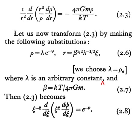
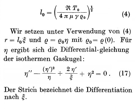
is the square of the isothermal sound speed. In their studies of pressure-bounded isothermal spheres, Ebert (1955, ZA, 37, 217) and Bonnor (1956, MNRAS, 116, 351) both started with this governing ODE, but developed its solution in different ways. Here we present both developments while highlighting transformations between the two.

Derivation by Bonnor (edited)	translation	Derivation by Ebert (edited)
	<math>G \Leftrightarrow \gamma</math>
	<math>\rho_c \Leftrightarrow \rho_0</math>
	<math>\frac{kT}{m} \Leftarrow c_s^2 \Rightarrow \frac{\Re T_0}{\mu}</math>
	<math>\beta^{1/2}\lambda^{-1/2} \Leftrightarrow l_0</math>
	<math>e^{-\psi} \Leftrightarrow \eta</math>

Both of these dimensionless governing ODEs — Bonnor's Eq. (2.8) and Ebert's Eq. (17) — are identical to the dimensionless expression derived by Emden (see the presentation elsewhere), namely,

<math> \frac{d^2v_1}{d\mathfrak{r}_1^2} +\frac{2}{\mathfrak{r}_1} \frac{dv_1}{dr} + e^{v_1} = 0 \, . </math>

The translation from Emden-to-Bonnor-to-Ebert is straightforward:

<math> \mathfrak{r}_1 = \xi|_\mathrm{Bonner} = \xi|_\mathrm{Ebert}~~~~\mathrm{and}~~~~e^{v_1} = e^{-\psi} = \eta \, . </math>

Related Wikipedia Discussions

• Bonnor-Ebert Mass

© 2014 - 2021 by Joel E. Tohline |   H_Book Home   |   YouTube   | Appendices: | Equations | Variables | References | Ramblings | Images | myphys.lsu | ADS | Recommended citation:   Tohline, Joel E. (2021), The Structure, Stability, & Dynamics of Self-Gravitating Fluids, a (MediaWiki-based) Vistrails.org publication, https://www.vistrails.org/index.php/User:Tohline/citation