Difference between revisions of "User:Tohline/Appendix/Ramblings/RiemannB74C692"
| Line 198: | Line 198: | ||
<table border="1" align="center" cellpadding="8"> | <table border="1" align="center" cellpadding="8"> | ||
<tr> | |||
<th align="center" colspan="4">''Direct''</th> | |||
</tr> | |||
<tr> | <tr> | ||
<td align="center">Model</td> | <td align="center">Model</td> | ||
<td align="center"> | <td align="center">λ<sub>EFE</sub></td> | ||
<td align="center">ΔT<sub>λ</sub></td> | <td align="center">ΔT<sub>λ</sub></td> | ||
<td align="center">1 Orbit</td> | <td align="center">1 Orbit</td> | ||
| Line 212: | Line 215: | ||
<tr> | <tr> | ||
<td align="center">b74c692</td> | <td align="center">b74c692</td> | ||
<td align="center"> | <td align="center">0.217773</td> | ||
<td align="center"> | <td align="center">0.3674</td> | ||
<td align="center"> | <td align="center">18.368</td> | ||
</tr> | </tr> | ||
<tr> | <tr> | ||
<td align="center">b90c333</td> | <td align="center">b90c333</td> | ||
<td align="center">- | <td align="center">-0.221411</td> | ||
<td align="center"> | <td align="center">0.3613</td> | ||
<td align="center"> | <td align="center">18.066</td> | ||
</tr> | </tr> | ||
<tr> | <tr> | ||
<td align="center">b28c256</td> | <td align="center">b28c256</td> | ||
<td align="center"> | <td align="center">0.020692</td> | ||
<td align="center"> | <td align="center">3.8662</td> | ||
<td align="center"> | <td align="center">193.31</td> | ||
</tr> | </tr> | ||
</table> | </table> | ||
Revision as of 21:40, 31 May 2020
Another S-type Example b74c692
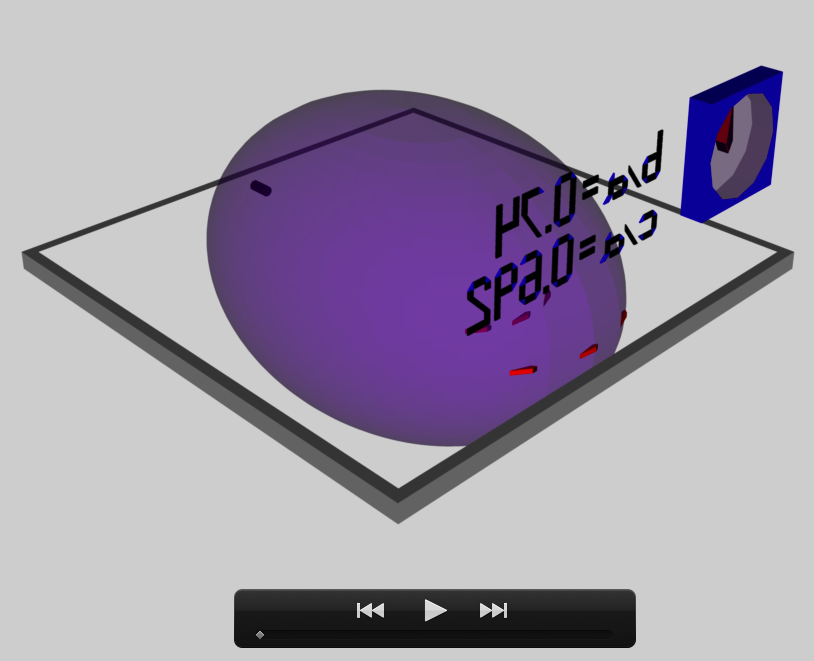
This chapter is an extension of the chapter we have titled, "Riemann Meets COLLADA & Oculus Rift S." In that chapter we used as our first example of a Riemann S-type ellipsoid the model with parameters, (b/a, c/a) = (0.41, 0.385). Here we construct a model with parameters, (b/a, c/a) = (0.74, 0.692). Other closely related chapters are listed below under the heading, "See Also".

|
|---|
| | Tiled Menu | Tables of Content | Banner Video | Tohline Home Page | |
Key Physical Parameters
The model that we have chosen to use in our second successful construction of a COLLADA-based, 3D and interactive animation has the following properties; this model has been selected from Table 2 of our accompanying discussion of Riemann S-type ellipsoids:
|
|
<math>~\frac{b}{a} = 0.74</math> |
|
||||
|
<math>~\frac{c}{a} = 0.692</math> |
||||||
|
Direct |
|
Adjoint |
||||
|
<math>~\Omega_\mathrm{EFE} = 0.638747</math> |
<math>~\Omega_\mathrm{EFE} = - 0.217773</math> |
|||||
|
<math>~\lambda_\mathrm{EFE} = 0.217773</math> |
<math>~\lambda_\mathrm{EFE} = - 0.638747 </math> |
|||||
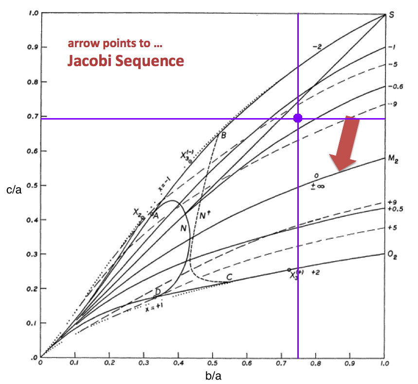
The subscript "EFE" on Ω and λ means that the relevant frequency is given in units that have been adopted in [EFE], that is, in units of <math>~[\pi G\rho]^{1 / 2}</math>. In Figure 1a, the solid purple circular marker (where the pair of purple lines cross) identifies the location of this model in the "c/a versus b/a" diagram that appears as Figure 2 on p. 902 of S. Chandrasekhar (1965); essentially the same diagram appears in §49 (p. 147) of [EFE].
Coding Steps
Here we begin with a working model of b41c385 and use incremental changes in the COLLADA-based code to construct a working model of b74c692.
- Pulling from the earlier modeling subsection titled, Final Touches …
-
Final17.dae TERRIFIC !:
Both hands of the clock now continue to cycle smoothly (through 9.126 "hours" = 9h 8m) while the laboratory frame completes 5.0 full spin periods — which will be 5.0 full spins of the ellipsoid as viewed from the inertial frame. This works in both visualization venues. -
Inertial17.dae:
This is identical to "Final17.dae" except that the system is viewed from the inertial frame of reference. This works in both visualization venues. -
[KEEP] Inertial21.dae:
Here, we set the "nudging" angle of the MidPlane to 0°, but moved the "nudging" angle of the ellipsoid from 0° to just 1°. This appears to work in both visualization venues.
-
Final17.dae TERRIFIC !:
- Pulling from a different earlier subsection titled, Multiple Lagrangian Fluid Elements …
-
MultiLagrange23.dae --> TestMulti23.dae:
This model shows the motion of nine (small, red cube) Lagrange particles whose motion is confined to the equatorial plane of the Riemann ellipsoid. This nicely illustrates that the volume occupied by a region of fluid remains unchanged as the fluid moves around the ellipsoid. This works in both visualization venues! -
[KEEP] MultiLagrange26.dae:
Here, we set the "nudging" angle of the MidPlane to 1°, and moved the "nudging" angle of the ellipsoid from 5° to 0°. Also, we bumped the purple's opacity up from 0.6 to 0.8. This appears to work in both visualization venues.
-
MultiLagrange23.dae --> TestMulti23.dae:
- TestMulti52.dae
Same as MultiLagrange23.dae --> TestMulti23.dae, except the starting ellipsoid angle is nudged by 45° instead of 5°. - [KEEP] TestMulti56.dae:
Same as MultiLagrange26.dae, except we have attempted to replace the alpha-numeric labeling. SUCCESS! Works in all three visualization venues: Mac "Preview", PC "3D Viewer", and Oculus RIft S. - Facebook glTF Transmutator (v1.5)
I am only now appreciating that, when a ".glb"-formatted file is imported into the Oculus Rift S inventory, the importation step is handled by Facebook's glTF Transmutator (v1.5). - TestMulti70b.dae
Same as TestMulti56.dae, except we have inserted the correct EllipsoidOctant geometries (drawn from b74c692 Old_DRot.dae). This works in both visualization venues.
Quantitative Animation
rotation_euler_Z
Whether the observer is viewing the system from an inertial frame of reference or a rotating frame of reference, this animation section specifies the rate at which the ellipsoid spins and the rate at which the "laboratory" is spinning. Three sets of data must be specified:
- The "First_rotation_euler_Z-input-array", which specifies TIME.
- The "First_rotation_euler_Z-output-array", which specifies how the ANGLE of orientation of the ellipsoid varies with TIME.
- The "Frame_rotation_euler_Z-output-array", which specifies how the spin ANGLE of the laboratory frame varies with TIME.
We have chosen to specify the time-varying angle in increments of 60° and to end the animation sequence after the ellipsoid (or, alternatively, the laboratory frame) has completed exactly five full spins. As a result — ignoring any zero-point offsets — one of the ANGLE arrays will vary from 0° to 5 × 360° = 1800° in 60° intervals (if spinning counter-clock-wise) or will vary from 1800° to 0° in -60° intervals (if spinning clock-wise). Again ignoring any zero-point offset, all the data values in the other ANGLE array will be 0°. The number of discrete data values that must be specified for each of the three arrays is therefore, by choice, count = (1800/60)+1 = 31.
All we have left to do is specify the TIME interval that is equivalent to a 60° turn of the ellipsoid, as viewed from the inertial frame of reference. Given that one cycle of the wall-clock's "minute" hand represents a frequency of <math>~[\pi G \rho]^{1 / 2}</math> and, furthermore by choice, we equate one cycle of the wall-clock's "minute" hand to TIME = 4 in COLLADA time units (approximately 4 seconds of real time), we know that one complete spin of the ellipsoid is equivalent to 4/|ΩEFE| units of TIME. Hence the ellipsoid will turn through 60° in a time, ΔTΩ = 4/[6|ΩEFE|] and it will take TIME = 20/|ΩEFE| to complete five full spins.
| Direct | |||
|---|---|---|---|
| Model | ΩEFE | ΔTΩ | 5 Spins |
| b41c385 | 0.547874 | 1.2168 | 36.505 |
| b74c692 | 0.638747 | 1.0437 | 31.311 |
| b90c333 | 0.447158 | 1.4909 | 44.727 |
| b28c256 | 0.456676 | 1.4598 | 43.795 |
location_X
Here we illustrate the motion of one Lagrangian fluid element as it moves along an elliptical path (b/a aspect ratio) in the equatorial plane of the Riemann ellipsoid. First we acknowledge that every fluid element completes one full orbit in a COLLADA-based time of, TIMEλ = 4/|λEFE|. Dividing the orbit into 50 equally spaced intervals of time therefore specifies a time increment, ΔTλ = 4/(50 |λEFE|). Drawing from a related accompanying discussion, we recognize that at each of these points in time — that is, for n = 1 → 50 — the x and y coordinate locations of the fluid element are given by the expressions,
|
<math>~x_n</math> |
<math>~= </math> |
<math>~\cos\biggl[-2\pi (n-1)\frac{\Delta T_\lambda}{4} \cdot \frac{\lambda_\mathrm{EFE}}{|\lambda_\mathrm{EFE}|}\biggr]</math> |
and |
<math>~y_n</math> |
<math>~= </math> |
<math>~\biggl(\frac{b}{a}\biggr)\sin\biggl[- 2\pi (n-1)\frac{\Delta T_\lambda}{4} \cdot \frac{\lambda_\mathrm{EFE}}{|\lambda_\mathrm{EFE}|}\biggr] \, ,</math> |
where we have assumed that the length of the longest axis of the ellipsoid is, a = 1. Note that, in the argument of these trigonometric functions, the sign of the frequency, λEFE, determines whether the fluid motion is regrograde (positive sign) or prograde (negative sign).
| Direct | |||
|---|---|---|---|
| Model | λEFE | ΔTλ | 1 Orbit |
| b41c385 | 0.079886 | 1.0014 | 50.071 |
| b74c692 | 0.217773 | 0.3674 | 18.368 |
| b90c333 | -0.221411 | 0.3613 | 18.066 |
| b28c256 | 0.020692 | 3.8662 | 193.31 |
COLLADA Model Files
b74c692DI.dae [Direct Inertial Frame] … a COLLADA code containing nnnn lines of <xml>-formatted ASCII text
<?xml version="1.0" encoding="UTF-8" standalone="no" ?>
b74c692DRot.dae [Direct Rotating Frame] … a COLLADA code containing nnnn lines of <xml>-formatted ASCII text
<?xml version="1.0" encoding="UTF-8" standalone="no" ?>
b74c692AI.dae [Adjunct Inertial Frame] … a COLLADA code containing nnnn lines of <xml>-formatted ASCII text
<?xml version="1.0" encoding="UTF-8" standalone="no" ?>
b74c692ARot.dae [Adjunct Rotating Frame] … a COLLADA code containing nnnn lines of <xml>-formatted ASCII text
<?xml version="1.0" encoding="UTF-8" standalone="no" ?>
See Also
- Discussion of Ou's Riemann-Like Ellipsoids
- Riemann Meets COLLADA & Oculus Rift S
- Virtual Reality and 3D Printing
- Success Importing Animated Scene into Oculus Rift S
- Carefully (Re)Build Riemann Type S Ellipsoids Inside Oculus Rift Environment: Example (b/a, c/a) = (0.41, 0.385)
- Other Example S-type Riemann Ellipsoids:

|
|---|
|
© 2014 - 2021 by Joel E. Tohline |

