Difference between revisions of "User:Tohline/SSC/Structure/IsothermalSphere"
| Line 7: | Line 7: | ||
<math>P = c_s^2 \rho \, ,</math> | <math>P = c_s^2 \rho \, ,</math> | ||
</div> | </div> | ||
where, <math>c_s</math> is the isothermal sound speed. Comparing this {{User:Tohline/Math/VAR_Pressure01}}-{{User:Tohline/Math/VAR_Density01}} relationship to | where, <math>~c_s</math> is the isothermal sound speed. Comparing this {{User:Tohline/Math/VAR_Pressure01}}-{{User:Tohline/Math/VAR_Density01}} relationship to | ||
<div align="center"> | <div align="center"> | ||
| Line 19: | Line 19: | ||
<math>c_s^2 = \frac{\Re T}{\bar{\mu}} = \frac{k T}{m_u \bar{\mu}} \, ,</math> | <math>c_s^2 = \frac{\Re T}{\bar{\mu}} = \frac{k T}{m_u \bar{\mu}} \, ,</math> | ||
</div> | </div> | ||
where, {{User:Tohline/Math/C_GasConstant}}, {{User:Tohline/Math/C_BoltzmannConstant}}, {{User:Tohline/Math/C_AtomicMassUnit}}, and {{User:Tohline/Math/MP_MeanMolecularWeight}} are all defined in the accompanying [[User:Tohline/Appendix/Variables_templates|variables appendix]]. It will be useful to note that, for an isothermal gas, {{User:Tohline/Math/VAR_Enthalpy01}} is related to {{User:Tohline/Math/VAR_Density01}} via the expression, | where, {{User:Tohline/Math/C_GasConstant}}, {{User:Tohline/Math/C_BoltzmannConstant}}, {{User:Tohline/Math/C_AtomicMassUnit}}, and {{User:Tohline/Math/MP_MeanMolecularWeight}} are all defined in the accompanying [[User:Tohline/Appendix/Variables_templates|variables appendix]]. It will be useful to note that, for an isothermal gas, the enthalpy, {{User:Tohline/Math/VAR_Enthalpy01}}, is related to {{User:Tohline/Math/VAR_Density01}} via the expression, | ||
<div align="center"> | <div align="center"> | ||
<math> | <math> | ||
| Line 25: | Line 26: | ||
</math> | </math> | ||
</div> | </div> | ||
==Governing Relations== | ==Governing Relations== | ||
Adopting [[User:Tohline/SphericallySymmetricConfigurations/SolutionStrategies#Technique_2|solution technique #2]], we need to solve the following second-order ODE relating the two unknown functions, {{User:Tohline/Math/VAR_Density01}} and {{User:Tohline/Math/VAR_Enthalpy01}}: | Adopting [[User:Tohline/SphericallySymmetricConfigurations/SolutionStrategies#Technique_2|solution technique #2]], we need to solve the following second-order ODE relating the two unknown functions, {{User:Tohline/Math/VAR_Density01}} and {{User:Tohline/Math/VAR_Enthalpy01}}: | ||
<div align="center"> | <div align="center"> | ||
<math>\frac{1}{r^2} \frac{d}{dr}\biggl( r^2 \frac{dH}{dr} \biggr) =- 4\pi G \rho</math> . | <math>\frac{1}{r^2} \frac{d}{dr}\biggl( r^2 \frac{dH}{dr} \biggr) =- 4\pi G \rho</math> . | ||
</div> | </div> | ||
Using the {{User:Tohline/Math/VAR_Enthalpy01}}-{{User:Tohline/Math/VAR_Density01}} relationship for an isothermal gas presented above, this can be rewritten entirely in terms of the density as, | Using the {{User:Tohline/Math/VAR_Enthalpy01}}-{{User:Tohline/Math/VAR_Density01}} relationship for an isothermal gas presented above, this can be rewritten entirely in terms of the density as, | ||
<div align="center"> | <div align="center"> | ||
<math>\frac{1}{r^2} \frac{d}{dr}\biggl( r^2 \frac{d\ln\rho}{dr} \biggr) =- \frac{4\pi G}{c_s^2} \rho \, ,</math> | <math>\frac{1}{r^2} \frac{d}{dr}\biggl( r^2 \frac{d\ln\rho}{dr} \biggr) =- \frac{4\pi G}{c_s^2} \rho \, ,</math> | ||
</div> | </div> | ||
<span id="keyExpression">or, equivalently,</span> | <span id="keyExpression">or, equivalently,</span> | ||
<div align="center"> | <div align="center"> | ||
| Line 42: | Line 48: | ||
</math> | </math> | ||
</div> | </div> | ||
where, | where, | ||
<div align="center"> | <div align="center"> | ||
<math> | <math> | ||
| Line 48: | Line 56: | ||
</math> | </math> | ||
</div> | </div> | ||
This matches the governing ODE whose derivation was published on p. 131 of [http://books.google.com/books?id=MiDQAAAAMAAJ&printsec=frontcover#v=onepage&q&f=true Robert Emden's (1907) book titled, ''Gaskugeln'']. | This matches the governing ODE whose derivation was published on p. 131 of [http://books.google.com/books?id=MiDQAAAAMAAJ&printsec=frontcover#v=onepage&q&f=true Robert Emden's (1907) book titled, ''Gaskugeln'']. | ||
| Line 74: | Line 83: | ||
</table> | </table> | ||
</div> | </div> | ||
By adopting the following dimensionless variables, | By adopting the following dimensionless variables, | ||
<div align="center"> | <div align="center"> | ||
<math> | <math> | ||
| Line 80: | Line 91: | ||
</math> | </math> | ||
</div> | </div> | ||
where <math>\rho_c</math> is the configuration's central density, the governing ODE can be rewritten in dimensionless form as, | |||
where <math>~\rho_c</math> is the configuration's central density, the governing ODE can be rewritten in dimensionless form as, | |||
<div align="center"> | <div align="center"> | ||
<math> | <math> | ||
| Line 86: | Line 99: | ||
</math> | </math> | ||
</div> | </div> | ||
which is exactly the equation numbered (II"a) that can be found on p. 133 of [http://books.google.com/books?id=MiDQAAAAMAAJ&printsec=frontcover#v=onepage&q&f=true Emden (1907)]. | which is exactly the equation numbered (II"a) that can be found on p. 133 of [http://books.google.com/books?id=MiDQAAAAMAAJ&printsec=frontcover#v=onepage&q&f=true Emden (1907)]. | ||
Emden numerically determined the behavior of the function <math>~v_1(\mathfrak{r}_1)</math>, its first derivative with respect to <math>~\mathfrak{r}_1</math>, <math>~v_1'</math>, along with <math>~e^{v_1}</math> and several other useful products, and published his results as Table 14, on p. 135 of his book. This table has been reproduced [[#Emden.27s_Numerical_Solution|immediately below]], primarily for historical purposes. | Emden numerically determined the behavior of the function <math>~v_1(\mathfrak{r}_1)</math>, its first derivative with respect to <math>~\mathfrak{r}_1</math>, <math>~v_1'</math>, along with <math>~e^{v_1}</math> and several other useful products, and published his results as Table 14, on p. 135 of his book. This table has been reproduced [[#Emden.27s_Numerical_Solution|immediately below]], primarily for historical purposes. | ||
| Line 134: | Line 148: | ||
A plot of <math>v_1</math> versus <math>\ln\mathfrak{r}_1</math>, as shown below in Figure 1a, translates into a log-log plot of the equilibrium configuration's <math>\rho(r)</math> density profile. Notice that this isolated isothermal configuration extends to infinity and that, at large radii, the density profile displays a simple power-law behavior — specifically, <math> \rho \propto r^{-2}</math>. This is consistent with our general discussion, [[User:Tohline/SSC/Structure/PowerLawDensity#Isothermal_Equation_of_State|presented elsewhere]], of power-law density distributions as solutions of the Lane-Emden equation. | A plot of <math>~v_1</math> versus <math>~\ln\mathfrak{r}_1</math>, as shown below in Figure 1a, translates into a log-log plot of the equilibrium configuration's <math>~\rho(r)</math> density profile. Notice that this isolated isothermal configuration extends to infinity and that, at large radii, the density profile displays a simple power-law behavior — specifically, <math>~ \rho \propto r^{-2}</math>. This is consistent with our general discussion, [[User:Tohline/SSC/Structure/PowerLawDensity#Isothermal_Equation_of_State|presented elsewhere]], of power-law density distributions as solutions of the Lane-Emden equation. | ||
| Line 155: | Line 169: | ||
<tr> | <tr> | ||
<td valign="top"> | <td valign="top"> | ||
(a) The <math>(x,y)</math> locations of the data points plotted in blue are drawn directly from column 1 and column 3 of Emden's Table 14 — specifically, <math>x = \ln(\mathfrak{r}_1)</math> and <math>y = v_1</math>. The dashed red line has a slope of <math>-2</math> and serves to illustrate that, at large radii, the [[User:Tohline/SSC/Structure/PowerLawDensity#Isothermal_Equation_of_State|isothermal density profile tends toward a <math>\rho \propto r^{-2}</math> distribution]]. | (a) The <math>~(x,y)</math> locations of the data points plotted in blue are drawn directly from column 1 and column 3 of Emden's Table 14 — specifically, <math>~x = \ln(\mathfrak{r}_1)</math> and <math>~y = v_1</math>. The dashed red line has a slope of <math>~-2</math> and serves to illustrate that, at large radii, the [[User:Tohline/SSC/Structure/PowerLawDensity#Isothermal_Equation_of_State|isothermal density profile tends toward a <math>~\rho \propto r^{-2}</math> distribution]]. | ||
</td> | </td> | ||
<td valign="top"> | <td valign="top"> | ||
(b) The <math>(x,y)</math> locations of the data points plotted in purple are drawn directly from column 1 and column 7 of Emden's Table 14 — specifically, <math>x = \ln(\mathfrak{r}_1)</math> and <math>y = \mathfrak{r}_1^2 v_1'</math>. The dashed green line has a slope of <math>+1</math> and serves to illustrate that, at large radii, the isothermal <math>M(r)</math> distribution tends toward a <math>M_r \propto r</math> distribution. | (b) The <math>~(x,y)</math> locations of the data points plotted in purple are drawn directly from column 1 and column 7 of Emden's Table 14 — specifically, <math>~x = \ln(\mathfrak{r}_1)</math> and <math>~y = \mathfrak{r}_1^2 v_1'</math>. The dashed green line has a slope of <math>~+1</math> and serves to illustrate that, at large radii, the isothermal <math>~M(r)</math> distribution tends toward a <math>~M_r \propto r</math> distribution. | ||
</td> | </td> | ||
</tr> | </tr> | ||
| Line 165: | Line 179: | ||
==Mass Profile== | ==Mass Profile== | ||
The mass enclosed within a given radius, <math>M_r</math>, can be determined by performing an appropriate volume-weighted integral over the density distribution. Specifically, based on the key expression for, | The mass enclosed within a given radius, <math>~M_r</math>, can be determined by performing an appropriate volume-weighted integral over the density distribution. Specifically, based on the key expression for, | ||
<div align="center"> | <div align="center"> | ||
| Line 175: | Line 189: | ||
<div align="center"> | <div align="center"> | ||
<math> | <math> | ||
M_r = \int_0^r 4\pi r^2 \rho(r) dr \, . | ~M_r = \int_0^r 4\pi r^2 \rho(r) dr \, . | ||
</math> | </math> | ||
</div> | </div> | ||
But <math>M_r</math> also can be determined from the information provided in column 7 of Emden's Table 14 — that is, from knowledge of the first derivative of <math>v_1</math>. The appropriate expression can be obtained from the mathematical prescription for | But <math>~M_r</math> also can be determined from the information provided in column 7 of Emden's Table 14 — that is, from knowledge of the first derivative of <math>~v_1</math>. The appropriate expression can be obtained from the mathematical prescription for | ||
<div align="center"> | <div align="center"> | ||
| Line 186: | Line 200: | ||
</div> | </div> | ||
in a spherically symmetric configuration. Since, for an isothermal equation of state (see above), | in a spherically symmetric configuration. Since, for an isothermal equation of state (see above), | ||
<div align="center"> | <div align="center"> | ||
<math> | <math> | ||
\frac{dP}{\rho} = c_s^2 {d\ln\rho} \, , | ~\frac{dP}{\rho} = c_s^2 {d\ln\rho} \, , | ||
</math> | </math> | ||
</div> | </div> | ||
the statement of hydrostatic balance can be rewritten as, | the statement of hydrostatic balance can be rewritten as, | ||
<div align="center"> | <div align="center"> | ||
<math> | <math> | ||
M_r = \frac{c_s^2}{G} \biggl[ - r^2 \frac{d\ln\rho}{dr} \biggr] = \frac{c_s^2}{G \rho_c^{1/2} \beta} \biggl[ - \mathfrak{r}_1^2 \frac{dv_1}{d\mathfrak{r}_1} \biggr] | ~M_r = \frac{c_s^2}{G} \biggl[ - r^2 \frac{d\ln\rho}{dr} \biggr] = \frac{c_s^2}{G \rho_c^{1/2} \beta} \biggl[ - \mathfrak{r}_1^2 \frac{dv_1}{d\mathfrak{r}_1} \biggr] | ||
= \biggl( \frac{c_s^6}{4\pi G^3 \rho_c} \biggr)^{1/2} \biggl[ - \mathfrak{r}_1^2 v_1' \biggr] \, . | = \biggl( \frac{c_s^6}{4\pi G^3 \rho_c} \biggr)^{1/2} \biggl[ - \mathfrak{r}_1^2 v_1' \biggr] \, . | ||
</math> | </math> | ||
</div> | </div> | ||
The quantity tabulated in column 7 of Emden's Table 14 is precisely the dimensionless term inside the square brackets of this last expression; having units of mass, the coefficient out front sets the mass scale of the equilibrium configuration and depends only on the choice of central density and isothermal sound speed. Hence, a plot of <math>\ln(\mathfrak{r}_1^2 v_1')</math> versus <math>\ln\mathfrak{r}_1</math>, as shown above in Figure 1b, translates into a log-log plot of the equilibrium configuration's <math>M_r</math> mass profile. Notice that, along with the radius, the mass of this isolated isothermal configuration extends to infinity and that, at large radii, the mass profile displays a simple power-law behavior — specifically, <math> M_r \propto r^{+1}</math>. | |||
The quantity tabulated in column 7 of Emden's Table 14 is precisely the dimensionless term inside the square brackets of this last expression; having units of mass, the coefficient out front sets the mass scale of the equilibrium configuration and depends only on the choice of central density and isothermal sound speed. Hence, a plot of <math>~\ln(\mathfrak{r}_1^2 v_1')</math> versus <math>~\ln\mathfrak{r}_1</math>, as shown above in Figure 1b, translates into a log-log plot of the equilibrium configuration's <math>~M_r</math> mass profile. Notice that, along with the radius, the mass of this isolated isothermal configuration extends to infinity and that, at large radii, the mass profile displays a simple power-law behavior — specifically, <math> ~M_r \propto r^{+1}</math>. | |||
As was realized independently by [http://adsabs.harvard.edu/abs/1955ZA.....37..217E Ebert (1955)] and [http://adsabs.harvard.edu/abs/1956MNRAS.116..351B Bonnor (1956)], a spherically symmetric isothermal equilibrium configuration of finite radius and finite mass can be constructed if the system is embedded in a pressure-confining external medium. We discuss their findings [[User:Tohline/SSC/Structure/BonnorEbert|elsewhere]]. | As was realized independently by [http://adsabs.harvard.edu/abs/1955ZA.....37..217E Ebert (1955)] and [http://adsabs.harvard.edu/abs/1956MNRAS.116..351B Bonnor (1956)], a spherically symmetric isothermal equilibrium configuration of finite radius and finite mass can be constructed if the system is embedded in a pressure-confining external medium. We discuss their findings [[User:Tohline/SSC/Structure/BonnorEbert|elsewhere]]. | ||
Revision as of 18:11, 8 March 2019
Isothermal Sphere

|
|---|
| | Tiled Menu | Tables of Content | Banner Video | Tohline Home Page | |
Here we supplement the simplified set of principal governing equations with an isothermal equation of state, that is, <math>~P</math> is related to <math>~\rho</math> through the relation,
<math>P = c_s^2 \rho \, ,</math>
where, <math>~c_s</math> is the isothermal sound speed. Comparing this <math>~P</math>-<math>~\rho</math> relationship to
Form A
of the Ideal Gas Equation of State,
|
<math>~P_\mathrm{gas} = \frac{\Re}{\bar{\mu}} \rho T</math> |
we see that,
<math>c_s^2 = \frac{\Re T}{\bar{\mu}} = \frac{k T}{m_u \bar{\mu}} \, ,</math>
where, <math>~\Re</math>, <math>~k</math>, <math>~m_u</math>, and <math>~\bar{\mu}</math> are all defined in the accompanying variables appendix. It will be useful to note that, for an isothermal gas, the enthalpy, <math>~H</math>, is related to <math>~\rho</math> via the expression,
<math> dH = \frac{dP}{\rho} = c_s^2 d\ln\rho \, . </math>
Governing Relations
Adopting solution technique #2, we need to solve the following second-order ODE relating the two unknown functions, <math>~\rho</math> and <math>~H</math>:
<math>\frac{1}{r^2} \frac{d}{dr}\biggl( r^2 \frac{dH}{dr} \biggr) =- 4\pi G \rho</math> .
Using the <math>~H</math>-<math>~\rho</math> relationship for an isothermal gas presented above, this can be rewritten entirely in terms of the density as,
<math>\frac{1}{r^2} \frac{d}{dr}\biggl( r^2 \frac{d\ln\rho}{dr} \biggr) =- \frac{4\pi G}{c_s^2} \rho \, ,</math>
or, equivalently,
<math> \frac{d^2\ln\rho}{dr^2} +\frac{2}{r} \frac{d\ln\rho}{dr} + \beta^2 \rho = 0 \, , </math>
where,
<math> \beta^2 \equiv \frac{4\pi G}{c_s^2} \, . </math>
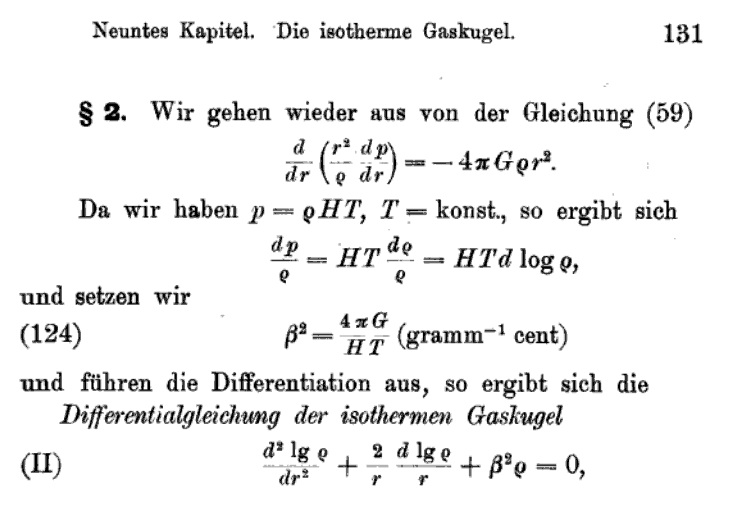
This matches the governing ODE whose derivation was published on p. 131 of Robert Emden's (1907) book titled, Gaskugeln.
|
Derivation by Emden (edited) |
|
|
Note that, in Emden's derivation, <math>H</math> is not enthalpy but, rather, the effective gas constant, <math>H = c_s^2/T</math>. |
|
By adopting the following dimensionless variables,
<math> \mathfrak{r}_1 \equiv \rho_c^{1/2} \beta r \, , ~~~~\mathrm{and}~~~~v_1 \equiv \ln(\rho/\rho_c) \, , </math>
where <math>~\rho_c</math> is the configuration's central density, the governing ODE can be rewritten in dimensionless form as,
<math> \frac{d^2v_1}{d\mathfrak{r}_1^2} +\frac{2}{\mathfrak{r}_1} \frac{dv_1}{d\mathfrak{r}_1} + e^{v_1} = 0 \, , </math>
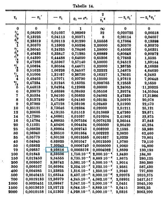
which is exactly the equation numbered (II"a) that can be found on p. 133 of Emden (1907). Emden numerically determined the behavior of the function <math>~v_1(\mathfrak{r}_1)</math>, its first derivative with respect to <math>~\mathfrak{r}_1</math>, <math>~v_1'</math>, along with <math>~e^{v_1}</math> and several other useful products, and published his results as Table 14, on p. 135 of his book. This table has been reproduced immediately below, primarily for historical purposes.
Note that a somewhat more extensive tabulation of the structural properties of isothermal spheres is provided by Chandrasekhar & Wares (1949, ApJ, 109, 551). In this published work as well as in §22 of Chapter IV in [C67], Chandrasekhar has written the governing ODE in a form that we will refer to as the,
Isothermal Lane-Emden Equation
|
<math>~\frac{1}{\xi^2} \frac{d}{d\xi}\biggl( \xi^2 \frac{d\psi}{d\xi} \biggr) = e^{-\psi}</math> |
It is straightforward to show that this is identical to Emden's governing expression after making the variable substitutions:
<math>~\mathfrak{r}_1 \rightarrow \xi</math> and <math>~v_1 \rightarrow -\psi </math>.
Across the astrophysics community, Chadrasekhar's notation has been widely — although not universally — adopted as the standard.
Emden's Numerical Solution
|
Note: The entry highlighted in blue in the <math>3^\mathrm{rd}</math> column must be a typesetting error. |
|
A more recent and more extensive tabulation of the structural properties of isothermal spheres is provided by:
An analytic — but approximate — solution to the isothermal Lane-Emden equation can be found:
|
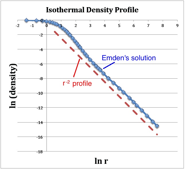
A plot of <math>~v_1</math> versus <math>~\ln\mathfrak{r}_1</math>, as shown below in Figure 1a, translates into a log-log plot of the equilibrium configuration's <math>~\rho(r)</math> density profile. Notice that this isolated isothermal configuration extends to infinity and that, at large radii, the density profile displays a simple power-law behavior — specifically, <math>~ \rho \propto r^{-2}</math>. This is consistent with our general discussion, presented elsewhere, of power-law density distributions as solutions of the Lane-Emden equation.
|
Figure 1: Emden's Numerical Solution |
|
|
(a) The <math>~(x,y)</math> locations of the data points plotted in blue are drawn directly from column 1 and column 3 of Emden's Table 14 — specifically, <math>~x = \ln(\mathfrak{r}_1)</math> and <math>~y = v_1</math>. The dashed red line has a slope of <math>~-2</math> and serves to illustrate that, at large radii, the isothermal density profile tends toward a <math>~\rho \propto r^{-2}</math> distribution. |
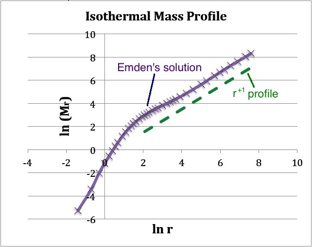
(b) The <math>~(x,y)</math> locations of the data points plotted in purple are drawn directly from column 1 and column 7 of Emden's Table 14 — specifically, <math>~x = \ln(\mathfrak{r}_1)</math> and <math>~y = \mathfrak{r}_1^2 v_1'</math>. The dashed green line has a slope of <math>~+1</math> and serves to illustrate that, at large radii, the isothermal <math>~M(r)</math> distribution tends toward a <math>~M_r \propto r</math> distribution. |
Mass Profile
The mass enclosed within a given radius, <math>~M_r</math>, can be determined by performing an appropriate volume-weighted integral over the density distribution. Specifically, based on the key expression for,
in spherically symmetric configurations, the relevant integral is,
<math> ~M_r = \int_0^r 4\pi r^2 \rho(r) dr \, . </math>
But <math>~M_r</math> also can be determined from the information provided in column 7 of Emden's Table 14 — that is, from knowledge of the first derivative of <math>~v_1</math>. The appropriate expression can be obtained from the mathematical prescription for
in a spherically symmetric configuration. Since, for an isothermal equation of state (see above),
<math> ~\frac{dP}{\rho} = c_s^2 {d\ln\rho} \, , </math>
the statement of hydrostatic balance can be rewritten as,
<math> ~M_r = \frac{c_s^2}{G} \biggl[ - r^2 \frac{d\ln\rho}{dr} \biggr] = \frac{c_s^2}{G \rho_c^{1/2} \beta} \biggl[ - \mathfrak{r}_1^2 \frac{dv_1}{d\mathfrak{r}_1} \biggr] = \biggl( \frac{c_s^6}{4\pi G^3 \rho_c} \biggr)^{1/2} \biggl[ - \mathfrak{r}_1^2 v_1' \biggr] \, . </math>
The quantity tabulated in column 7 of Emden's Table 14 is precisely the dimensionless term inside the square brackets of this last expression; having units of mass, the coefficient out front sets the mass scale of the equilibrium configuration and depends only on the choice of central density and isothermal sound speed. Hence, a plot of <math>~\ln(\mathfrak{r}_1^2 v_1')</math> versus <math>~\ln\mathfrak{r}_1</math>, as shown above in Figure 1b, translates into a log-log plot of the equilibrium configuration's <math>~M_r</math> mass profile. Notice that, along with the radius, the mass of this isolated isothermal configuration extends to infinity and that, at large radii, the mass profile displays a simple power-law behavior — specifically, <math> ~M_r \propto r^{+1}</math>.
As was realized independently by Ebert (1955) and Bonnor (1956), a spherically symmetric isothermal equilibrium configuration of finite radius and finite mass can be constructed if the system is embedded in a pressure-confining external medium. We discuss their findings elsewhere.
Summary
Based on the above derivations, the internal structural properties of an equilibrium isothermal sphere can be described in terms of the tabulated quantities provided in Emden's Table 14 as follows:
- Radial Coordinate Position:
- Given the isothermal sound speed, <math>c_s</math>, and the central density, <math>\rho_c</math>, the radial coordinate is,
<math>r = ( \rho_c \beta^2 )^{-1/2} \mathfrak{r}_1 = \biggl( \frac{c_s^2}{4\pi G \rho_c} \biggr)^{1/2} \mathfrak{r}_1 </math> .
- Density & Pressure:
- As a function of the radial coordinate, <math>r(\mathfrak{r}_1)</math>, the density profile is,
<math>\rho(r(\mathfrak{r}_1))= \rho_c e^{v_1(\mathfrak{r}_1)}</math>;
- and the pressure profile is,
<math>P(r(\mathfrak{r}_1))= (c_s^2 \rho_c) e^{v_1(\mathfrak{r}_1)}</math>.
- As has been explicitly pointed out in the above discussion associated with Figure 1a, the density profile — and, hence, also the pressure profile — extends to infinity and, at large radii, behaves as a power law; specifically, <math>\rho \propto r^{-2}</math>.
- Mass:
- Given <math>c_s</math> and <math>\rho_c</math>, the natural mass scale is,
<math>M_0 \equiv \biggl( \frac{c_s^6}{4\pi G^3 \rho_c} \biggr)^{1/2} </math> ;
- and, expressed in terms of <math>M_0</math>, the mass that lies interior to radius <math>r</math> is,
<math> M_r = M_0 [ - \mathfrak{r}_1^2 v_1' ] \, . </math>
- As discussed above in the context of Figure 1b, at large radii, the mass increases linearly with <math>r</math>. Because the density and pressure profiles extend to infinity, this means that the mass of an isolated isothermal sphere is infinite.
- Enthalpy & Gravitational Potential:
- To within an additive constant, the enthalpy distribution is,
<math>H(r(\mathfrak{r}_1))= c_s^2 [- v_1(\mathfrak{r}_1)]</math>;
- and the gravitational potential is,
<math>\Phi(r(\mathfrak{r}_1)) = - H(r(\mathfrak{r}_1))= c_s^2 v_1(\mathfrak{r}_1)</math>.
- Mean-to-Local Density Ratio:
- The ratio of the configuration's mean density, inside a given radius, to its local density at that radius is,
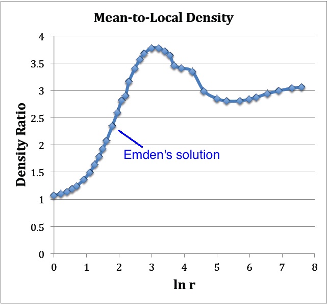
<math>\frac{\bar{\rho}}{\rho} = \frac{3M_r}{4\pi r^3 \rho} = 3\biggl[- \frac{v_1'}{\mathfrak{r}_1 e^{v_1}} \biggr] </math> .
- As Figure 2 shows, at large <math>r</math> this density ratio goes to the value of 3, which means that the term inside the square brackets goes to unity at large <math>r</math>. This behavior is consistent with the limiting power-law behavior of both <math>M_r</math> and <math>\rho</math>, discussed above.
|
Figure 2: From Emden's Tabulated Data |
|
The blue curve displays an evaluation of the density ratio, <math>[- 3v_1'/(\mathfrak{r}_1 e^{v_1}) ]</math>, as a function of <math>\ln (\mathfrak{r}_1)</math>, as determined from the data presented in Emden's Table 14, shown above. |
Our Numerical Integration
The above governing relation — see especially Chandrasekhar's notation — may be rewritten as (see also, for example, §19.8, eq. 19.35 of [KW94]),
|
<math>~\frac{d^2w}{dr^2} +\frac{2}{r} \frac{d w}{dr} </math> |
<math>~=</math> |
<math>~e^{-w} \, ,</math> |
where we appreciate that,
<math>~w \equiv \ln\biggl(\frac{\rho}{\rho_c}\biggr) \, .</math>
We'll adopt the following finite-difference approximations for the first and second derivatives on a grid of radial spacing, <math>~\Delta_r</math>:
|
<math>~w_i'</math> |
<math>~\approx</math> |
<math>~\frac{w_+ - w_-}{2\Delta_r}</math> |
and,
|
<math>~w_i</math> |
<math>~\approx</math> |
<math>~\frac{w_+ - 2w_i +w_-}{\Delta_r^2} \, .</math> |
Our finite-difference approximation of the governing equation is, then,
|
<math>~r_i \biggl[ \frac{w_+ - 2w_i +w_-}{\Delta_r^2} \biggr] + 2\biggl[ \frac{w_+ - w_-}{2\Delta_r} \biggr] </math> |
<math>~=</math> |
<math>~r_i e^{-w_i} </math> |
|
<math>~\Rightarrow ~~~ r_i [ w_+ - 2w_i +w_- ] + \Delta_r [ w_+ - w_- ] </math> |
<math>~=</math> |
<math>~\Delta_r^2 r_i e^{-w_i} </math> |
|
<math>~\Rightarrow ~~~w_+ </math> |
<math>~=</math> |
<math>~\frac{\Delta_r^2 r_i e^{-w_i} + 2r_i w_i + w_- (\Delta_r - r_i)}{( \Delta_r + r_i)} \, .</math> |
Now, for the first two steps away from the center — where, <math>~w_i = w_0 = 0</math> and <math>~r_i = r_0 = 0</math> — we will use the following power-series expansion (see, for example, eq. 377 from §22 in Chapter IV of [C67]) to determine the value of <math>~w_i</math>:
|
<math>~w_1 </math> |
<math>~=</math> |
<math>~\frac{\Delta_r^2}{6} - \frac{\Delta_r^4}{120} + \frac{\Delta_r^6}{1890} \, ,</math> |
and,
|
<math>~w_2 </math> |
<math>~=</math> |
<math>~\frac{(2\Delta_r)^2}{6} - \frac{(2\Delta_r)^4}{120} + \frac{(2\Delta_r)^6}{1890} \, .</math> |
Related Wikipedia Discussions

|
|---|
|
© 2014 - 2021 by Joel E. Tohline |

