Difference between revisions of "User:Tohline/SSC/Structure/BiPolytropes/Analytic5 1"
(→Expression for Free Energy: fix a few things) |
|||
| Line 1,612: | Line 1,612: | ||
(Apology: The parameter <math>~x_i</math> introduced here is identical to the parameter <math>~\ell_i</math> that was introduced earlier in the context of [[User:Tohline/SSC/Structure/BiPolytropes/Analytic5_1#Limiting_Mass|our discussion of the "Limiting Mass"]] of these models. Sorry for the unnecessary duplication of parameters and possible confusion!) | (Apology: The parameter <math>~x_i</math> introduced here is identical to the parameter <math>~\ell_i</math> that was introduced earlier in the context of [[User:Tohline/SSC/Structure/BiPolytropes/Analytic5_1#Limiting_Mass|our discussion of the "Limiting Mass"]] of these models. Sorry for the unnecessary duplication of parameters and possible confusion!) | ||
<table border="1" align="center" width=" | <div id="Buchdahl1978"> | ||
<table border="1" align="center" width="85%" cellpadding="8"> | |||
<tr><td align="left"> | <tr><td align="left"> | ||
While our aim, here, has been to determine an expression for the gravitational potential energy of a ''truncated'' <math>~n = 5</math> polytropic sphere, our derived expression can also give the gravitational potential of an ''isolated'' <math>~n = 5</math> polytrope by evaluating the expression in the limit <math>~x_i \rightarrow \infty</math>. In this limit, the first term inside the square brackets goes to zero, while the second term, | While our aim, here, has been to determine an expression for the gravitational potential energy of a ''truncated'' <math>~n = 5</math> polytropic sphere, our derived expression can also give the gravitational potential of an ''isolated'' <math>~n = 5</math> polytrope by evaluating the expression in the limit <math>~x_i \rightarrow \infty</math>. In this limit, the first term inside the square brackets goes to zero, while the second term, | ||
| Line 1,688: | Line 1,689: | ||
<div align="center"> | <div align="center"> | ||
<table border="1" align="center" cellpadding="8"> | <table border="1" align="center" cellpadding="8" width="75%"> | ||
<tr><td align="center"> | <tr><td align="center"> | ||
Equation Excerpt from | Equation Excerpt from | ||
| Line 1,704: | Line 1,705: | ||
</td></tr> | </td></tr> | ||
</table> | </table> | ||
</div> | |||
Notice that these two terms combine to give, for the core, | Notice that these two terms combine to give, for the core, | ||
Revision as of 16:25, 13 April 2015
BiPolytrope with <math>n_c = 5</math> and <math>n_e=1</math>

|
|---|
| | Tiled Menu | Tables of Content | Banner Video | Tohline Home Page | |
Here we construct a bipolytrope in which the core has an <math>n_c=5</math> polytropic index and the envelope has an <math>n_c=1</math> polytropic index. This system is particularly interesting because the entire structure can be described by closed-form, analytic expressions. In deriving the properties of this model, we will follow the general solution steps for constructing a bipolytrope that we have outlined elsewhere. [On 30 March 2013, J. E. Tohline wrote: As far as I have been able to determine, this analytic structural model has not previously been published in a refereed, archival journal.] [On 23 June 2013, J. E. Tohline wrote: Last night I stumbled upon an article by Eagleton, Faulkner, and Cannon (1998, MNRAS, 298, 831) in which this identical analytically definable bipolytrope has been presented. Insight drawn from this article is presented in an additional subsection, below.]
Steps 2 & 3
Based on the discussion presented elsewhere of the structure of an isolated <math>n=5</math> polytrope, the core of this bipolytrope will have the following properties:
<math> \theta(\xi) = \biggl[ 1 + \frac{1}{3}\xi^2 \biggr]^{-1/2} ~~~~\Rightarrow ~~~~ \theta_i = \biggl[ 1 + \frac{1}{3}\xi_i^2 \biggr]^{-1/2} ; </math>
<math> \frac{d\theta}{d\xi} = - \frac{\xi}{3}\biggl[ 1 + \frac{1}{3}\xi^2 \biggr]^{-3/2} ~~~~\Rightarrow ~~~~ \biggl(\frac{d\theta}{d\xi}\biggr)_i = - \frac{\xi_i}{3}\biggl[ 1 + \frac{1}{3}\xi_i^2 \biggr]^{-3/2} \, . </math>
The first zero of the function <math>\theta(\xi)</math> and, hence, the surface of the corresponding isolated <math>n=5</math> polytrope is located at <math>\xi_s = \infty</math>. Hence, the interface between the core and the envelope can be positioned anywhere within the range, <math>0 < \xi_i < \infty</math>.
Step 4: Throughout the core (<math>0 \le \xi \le \xi_i</math>)
|
Specify: <math>K_c</math> and <math>\rho_0 ~\Rightarrow</math> |
|
|||
|
<math>\rho</math> |
<math>=</math> |
<math>\rho_0 \theta^{n_c}</math> |
<math>=</math> |
<math>\rho_0 \biggl( 1 + \frac{1}{3}\xi^2 \biggr)^{-5/2}</math> |
|
<math>P</math> |
<math>=</math> |
<math>K_c \rho_0^{1+1/n_c} \theta^{n_c + 1}</math> |
<math>=</math> |
<math>K_c \rho_0^{6/5} \biggl( 1 + \frac{1}{3}\xi^2 \biggr)^{-3}</math> |
|
<math>r</math> |
<math>=</math> |
<math>\biggl[ \frac{(n_c + 1)K_c}{4\pi G} \biggr]^{1/2} \rho_0^{(1-n_c)/(2n_c)} \xi</math> |
<math>=</math> |
<math>\biggl[ \frac{K_c}{G\rho_0^{4/5}} \biggr]^{1/2} \biggl(\frac{3}{2\pi}\biggr)^{1/2} \xi</math> |
|
<math>M_r</math> |
<math>=</math> |
<math>4\pi \biggl[ \frac{(n_c + 1)K_c}{4\pi G} \biggr]^{3/2} \rho_0^{(3-n_c)/(2n_c)} \biggl(-\xi^2 \frac{d\theta}{d\xi} \biggr)</math> |
<math>=</math> |
<math>\biggl[ \frac{K_c^3}{G^3 \rho_0^{2/5} } \biggr]^{1/2} \biggl( \frac{2\cdot 3}{\pi } \biggr)^{1/2} \biggl[ \xi^3 \biggl( 1 + \frac{1}{3}\xi^2 \biggr)^{-3/2} \biggr]</math> |
Step 5: Interface Conditions
|
|
Setting <math>n_c=5</math>, <math>n_e=1</math>, and <math>\phi_i = 1 ~~~~\Rightarrow</math> |
|||
|
<math>\frac{\rho_e}{\rho_0}</math> |
<math>=</math> |
<math>\biggl( \frac{\mu_e}{\mu_c} \biggr) \theta^{n_c}_i \phi_i^{-n_e}</math> |
<math>=</math> |
<math>\biggl( \frac{\mu_e}{\mu_c} \biggr) \theta^{5}_i </math> |
|
<math>\biggl( \frac{K_e}{K_c} \biggr) </math> |
<math>=</math> |
<math>\rho_0^{1/n_c - 1/n_e}\biggl( \frac{\mu_e}{\mu_c} \biggr)^{-(1+1/n_e)} \theta^{1 - n_c/n_e}_i</math> |
<math>=</math> |
<math>\rho_0^{-4/5}\biggl( \frac{\mu_e}{\mu_c} \biggr)^{-2} \theta^{-4}_i</math> |
|
<math>\frac{\eta_i}{\xi_i}</math> |
<math>=</math> |
<math>\biggl[ \frac{n_c + 1}{n_e+1} \biggr]^{1/2} \biggl( \frac{\mu_e}{\mu_c}\biggr) \theta_i^{(n_c-1)/2} \phi_i^{(1-n_e)/2}</math> |
<math>=</math> |
<math>3^{1/2} \biggl( \frac{\mu_e}{\mu_c}\biggr) \theta_i^{2}</math> |
|
<math>\biggl( \frac{d\phi}{d\eta} \biggr)_i</math> |
<math>=</math> |
<math>\biggl[ \frac{n_c + 1}{n_e + 1} \biggr]^{1/2} \theta_i^{- (n_c + 1)/2} \phi_i^{(n_e+1)/2} \biggl( \frac{d\theta}{d\xi} \biggr)_i</math> |
<math>=</math> |
<math>3^{1/2} \theta_i^{- 3} \biggl( \frac{d\theta}{d\xi} \biggr)_i</math> |
Step 6: Envelope Solution
Adopting equation (8) of Beech (1988), the most general solution to the <math>n=1</math> Lane-Emden equation can be written in the form,
<math> \phi = A \biggl[ \frac{\sin(\eta - B)}{\eta} \biggr] \, , </math>
where <math>A</math> and <math>B</math> are constants. The first derivative of this function is,
<math> \frac{d\phi}{d\eta} = \frac{A}{\eta^2} \biggl[ \eta\cos(\eta-B) - \sin(\eta-B) \biggr] \, . </math>
From Step 5, above, we know the value of the function, <math>\phi</math> and its first derivative at the interface; specifically,
<math> \phi_i = 1~~~~\mathrm{and} ~~~~\biggl( \frac{d\phi}{d\eta}\biggr)_i =3^{1/2} \theta_i^{- 3} \biggl( \frac{d\theta}{d\xi} \biggr)_i~~~~ \mathrm{at}~~~~\eta_i =3^{1/2} \xi_i \biggl( \frac{\mu_e}{\mu_c}\biggr) \theta_i^{2}</math>
From this information we can determine the constants <math>A</math> and <math>B</math>; specifically,
<math> \eta_i - B = \tan^{-1}(\Lambda_i^{-1}) = \frac{\pi}{2}- \tan^{-1}(\Lambda_i) \, , </math>
<math> A = \frac{\phi_i \eta_i}{\sin(\eta_i - B)} = \phi_i \eta_i (1 + \Lambda_i^2)^{1/2} \, , </math>
where,
<math> \Lambda_i = \frac{1}{\eta_i} + \frac{1}{\phi_i} \biggl(\frac{d\phi}{d\eta}\biggr)_i \, . </math>
Step 7
The surface will be defined by the location, <math>\eta_s</math>, at which the function <math>\phi(\eta)</math> first goes to zero, that is,
<math> \eta_s = \pi + B = \frac{\pi}{2} + \eta_i + \tan^{-1}(\Lambda_i) \, . </math>
Step 8: Throughout the envelope (<math>\eta_i \le \eta \le \eta_s</math>)
|
|
Knowing: <math>K_e/K_c</math> and <math>\rho_e/\rho_0</math> from Step 5 <math>\Rightarrow</math> |
|||||
|
<math>\rho</math> |
<math>=</math> |
<math>\rho_e \phi^{n_e}</math> |
<math>=</math> |
<math>\rho_0 \biggl(\frac{\rho_e}{\rho_0}\biggr) \phi</math> |
<math>=</math> |
<math>\rho_0 \biggl( \frac{\mu_e}{\mu_c} \biggr) \theta^{5}_i \phi</math> |
|
<math>P</math> |
<math>=</math> |
<math>K_e \rho_e^{1+1/n_e} \phi^{n_e + 1}</math> |
<math>=</math> |
<math>K_c \rho_0^{6/5} \biggl(\frac{K_e \rho_0^{4/5}}{K_c}\biggr) \biggl(\frac{\rho_e}{\rho_0}\biggr)^{2} \phi^{2}</math> |
<math>=</math> |
<math>K_c \rho_0^{6/5} \theta^{6}_i \phi^{2}</math> |
|
<math>r</math> |
<math>=</math> |
<math>\biggl[ \frac{(n_e + 1)K_e}{4\pi G} \biggr]^{1/2} \rho_e^{(1-n_e)/(2n_e)} \eta</math> |
<math>=</math> |
<math>\biggl[ \frac{K_c}{G \rho_0^{4/5}} \biggr]^{1/2} \biggl( \frac{K_e \rho_0^{4/5}}{K_c} \biggr)^{1/2} (2\pi)^{-1/2}\eta</math> |
<math>=</math> |
<math>\biggl[ \frac{K_c}{G \rho_0^{4/5}} \biggr]^{1/2} \biggl( \frac{\mu_e}{\mu_c} \biggr)^{-1} \theta^{-2}_i (2\pi)^{-1/2}\eta</math> |
|
<math>M_r</math> |
<math>=</math> |
<math>4\pi \biggl[ \frac{(n_e + 1)K_e}{4\pi G} \biggr]^{3/2} \rho_e^{(3-n_e)/(2n_e)} \biggl(-\eta^2 \frac{d\phi}{d\eta} \biggr)</math> |
<math>=</math> |
<math>\biggl[ \frac{K_c^3}{G^3 \rho_0^{2/5}} \biggr]^{1/2} \biggl( \frac{K_e \rho_0^{4/5}}{K_c} \biggr)^{3/2} \biggl(\frac{\rho_e}{\rho_0}\biggr) \biggl( \frac{2}{\pi} \biggr)^{1/2} \biggl(-\eta^2 \frac{d\phi}{d\eta} \biggr)</math> |
<math>=</math> |
<math>\biggl[ \frac{K_c^3}{G^3 \rho_0^{2/5}} \biggr]^{1/2} \biggl( \frac{\mu_e}{\mu_c} \biggr)^{-2} \theta^{-1}_i \biggl( \frac{2}{\pi} \biggr)^{1/2} \biggl(-\eta^2 \frac{d\phi}{d\eta} \biggr)</math> |
Examples
Normalization
The dimensionless variables used in Tables 1 & 2 are defined as follows:
|
<math>\rho^*</math> |
<math>\equiv</math> |
<math>\frac{\rho}{\rho_0}</math> |
; |
<math>r^*</math> |
<math>\equiv</math> |
<math>\frac{r}{[K_c^{1/2}/(G^{1/2}\rho_0^{2/5})]}</math> |
|
<math>P^*</math> |
<math>\equiv</math> |
<math>\frac{P}{K_c\rho_0^{6/5}}</math> |
; |
<math>M_r^*</math> |
<math>\equiv</math> |
<math>\frac{M_r}{[K_c^{3/2}/(G^{3/2}\rho_0^{1/5})]}</math> |
|
<math>H^*</math> |
<math>\equiv</math> |
<math>\frac{H}{K_c\rho_0^{1/5}}</math> |
. |
|
||
Parameter Values
The <math>2^\mathrm{nd}</math> column of Table 1 catalogues the analytic expressions that define various parameters and physical properties (as identified, respectively, in column 1) of the <math>n_c=5</math>, <math>n_e=1</math> bipolytrope. We have evaluated these expressions for various choices of the dimensionless interface radius, <math>\xi_i</math>, and have tabulated the results in the last few columns of the table. The tabulated values have been derived assuming <math>\mu_e/\mu_c = 1</math>, that is, assuming that the core and the envelope have the same mean molecular weights.
Table 1: Properties of <math>n_c=5</math>, <math>n_e=1</math>, BiPolytrope Having Various Interface Locations, <math>\xi_i</math>
File:BiPolytropeParametersV01.xml
|
Parameter |
<math>\xi_i</math> |
0.5 |
1.0 |
3.0 |
|
<math>\theta_i</math> |
<math>\biggl( 1+\frac{1}{3}\xi_i^2 \biggr)^{-1/2}</math> |
0.96077 |
0.86603 |
0.50000 |
|
<math>-\biggl(\frac{d\theta_i}{d\xi}\biggr)_i</math> |
<math>\frac{1}{3} \xi_i \biggl( 1+\frac{1}{3}\xi_i^2 \biggr)^{-3/2}</math> |
0.14781 |
0.21651 |
0.12500 |
|
<math>r^*_\mathrm{core} \equiv r^*_i</math> |
<math>\biggl( \frac{3}{2\pi} \biggr)^{1/2} \xi_i</math> |
0.34549 |
0.69099 |
2.07297 |
|
<math>\rho^*_i \biggr|_c = \biggl( \frac{\mu_e}{\mu_c} \biggr)^{-1} \rho^*_i \biggr|_e</math> |
<math>\biggl( 1+\frac{1}{3}\xi_i^2 \biggr)^{-5/2}</math> |
0.81864 |
0.48714 |
0.03125 |
|
<math>P^*_i</math> |
<math>\biggl( 1+\frac{1}{3}\xi_i^2 \biggr)^{-3}</math> |
0.78653 |
0.42188 |
0.01563 |
|
<math>H^*_i \biggr|_c = \frac{n_c+1}{n_e+1} \biggl( \frac{\mu_e}{\mu_c} \biggr) H^*_i \biggr|_e</math> |
<math>6 \biggl( 1+\frac{1}{3}\xi_i^2 \biggr)^{-1/2}</math> |
5.76461 |
5.19615 |
3.00000 |
|
<math>M^*_\mathrm{core}</math> |
<math>\biggl( \frac{6}{\pi}\biggr)^{1/2} (\xi_i \theta_i)^3</math> |
0.15320 |
0.89762 |
4.66417 |
|
<math>\biggl( \frac{\mu_e}{\mu_c} \biggr)^{-1}\eta_i</math> |
<math>\sqrt{3} ~\theta_i^2 \xi_i</math> |
0.79941 |
1.29904 |
1.29904 |
|
<math>-\biggl( \frac{d\phi}{d\eta} \biggr)_i</math> |
<math>\sqrt{3} ~\theta_i^{-3} \biggl( - \frac{d\theta}{d\xi} \biggr)_i = \frac{\xi_i}{\sqrt{3}}</math> |
0.28868 |
0.57735 |
1.73205 |
|
<math>\Lambda_i</math> |
<math>\frac{1}{\eta_i} + \biggl( \frac{d\phi}{d\eta} \biggr)_i</math> |
0.96225 |
0.19245 |
-0.96225 |
|
<math>A</math> |
<math>\eta_i (1 + \Lambda_i^2)^{1/2}</math> |
1.10940 |
1.32288 |
1.80278 |
|
<math>B</math> |
<math>\eta_i - \frac{\pi}{2} + \tan^{-1}( \Lambda_i)</math> |
- 0.00523 |
-0.08163 |
-1.03792 |
|
<math>\eta_s</math> |
<math>\pi + B</math> |
3.13637 |
3.05996 |
2.10367 |
|
<math>- \biggl( \frac{d\phi}{d\eta} \biggr)_s</math> |
<math>\frac{A}{\eta_s}</math> |
0.35372 |
0.43232 |
0.85697 |
|
<math>\biggl( \frac{\mu_e}{\mu_c} \biggr) \cdot \biggl[ R^* \equiv r^*_s \biggr]</math> |
<math>\frac{\eta_s}{\sqrt{2\pi} ~\theta_i^2}</math> |
1.35550 |
1.62766 |
3.35697 |
|
<math>\biggl( \frac{\mu_e}{\mu_c} \biggr)^2 M^*_\mathrm{tot}</math> |
<math>\biggl(\frac{2}{\pi}\biggr)^{1/2} \theta_i^{-1} \biggl( -\eta^2 \frac{d\phi}{d\eta} \biggr)_s = \biggl(\frac{2}{\pi}\biggr)^{1/2} \frac{A\eta_s}{\theta_i}</math> |
2.88959 |
3.72945 |
6.05187 |
|
<math>\biggl(\frac{\mu_e}{\mu_c}\biggr)^{-2} \cdot \biggl[ \nu \equiv \frac{M_\mathrm{core}}{M_\mathrm{tot}} \biggr]</math> |
<math>\sqrt{3} ~\biggl( \frac{\xi_i^3 \theta_i^4}{A\eta_s} \biggr)</math> |
0.05302 |
0.24068 |
0.77070 |
|
<math>\biggl(\frac{\mu_e}{\mu_c}\biggr)^{-1} \cdot \biggl[ q \equiv \frac{r_\mathrm{core}}{R} \biggr]</math> |
<math>\sqrt{3}~\biggl[\frac{\xi_i \theta_i^2}{\eta_s}\biggr]</math> |
0.25488 |
0.42453 |
0.61751 |
Profile
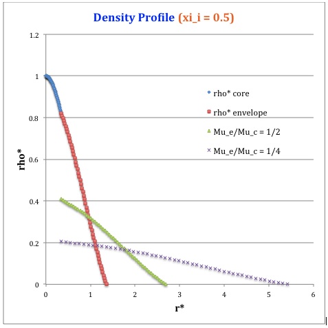
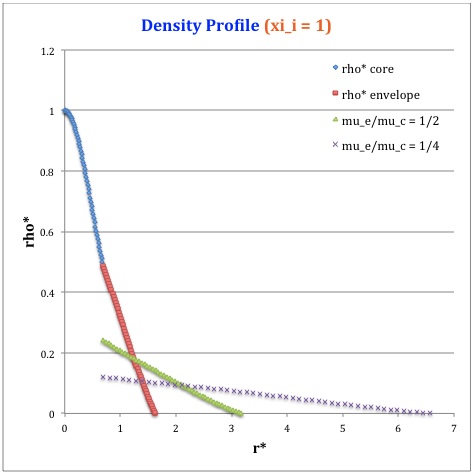
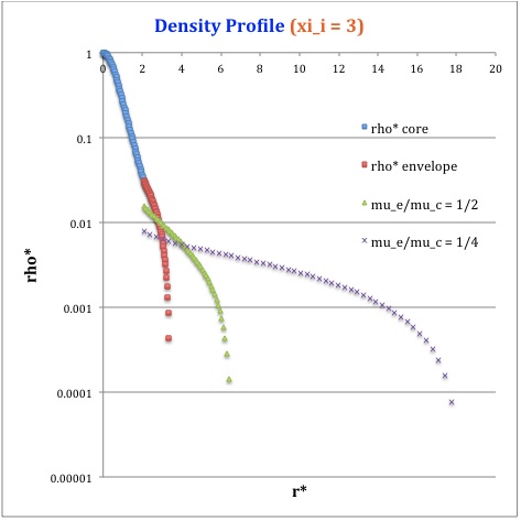
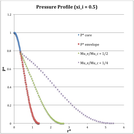
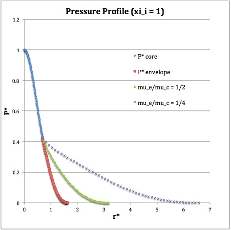
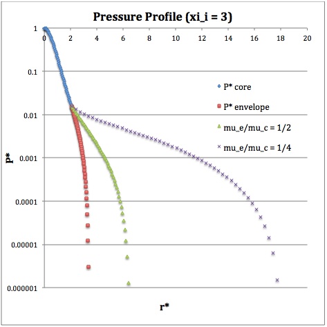
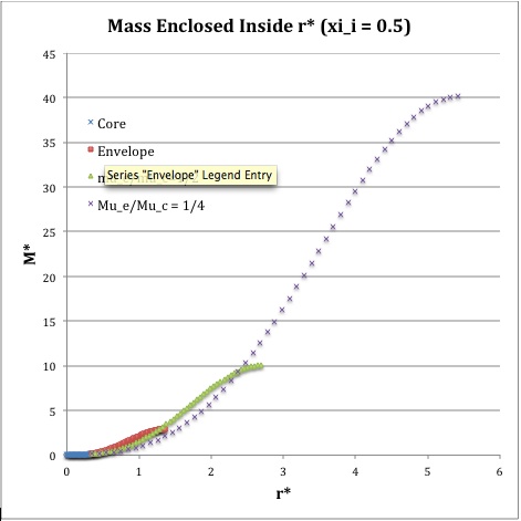
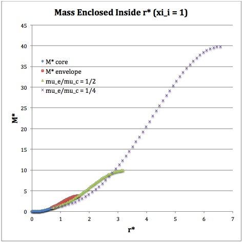
Once the values of the key set of parameters have been determined as illustrated in Table 1, the radial profile of various physical variables can be determined throughout the bipolytrope as detailed in step #4 and step #8, above. Table 2 summarizes the mathematical expressions that define the profile throughout the core (column 2) and throughout the envelope (column 3) of the normalized mass density, <math>\rho^*(r^*)</math>, the normalized gas pressure, <math>P^*(r^*)</math>, and the normalized mass interior to <math>r^*</math>, <math>M_r^*(r^*)</math>. For all profiles, the relevant normalized radial coordinate is <math>r^*</math>, as defined in the <math>2^\mathrm{nd}</math> row of Table 2. Graphical illustrations of these resulting profiles can be viewed by clicking on the thumbnail images posted in the last few columns of Table 2.
Table 2: Radial Profile of Various Physical Variables
|
Variable |
Throughout the Core |
Throughout the Envelope† |
Plotted Profiles |
||
|
<math>\xi_i = 0.5</math> |
<math>\xi_i = 1.0</math> |
<math>\xi_i = 3.0</math> |
|||
|
<math>r^*</math> |
<math>\biggl( \frac{3}{2\pi} \biggr)^{1/2} \xi</math> |
<math>\biggl( \frac{\mu_e}{\mu_c} \biggr)^{-1} \theta^{-2}_i (2\pi)^{-1/2}\eta</math> |
|
||
|
<math>\rho^*</math> |
<math>\biggl( 1 + \frac{1}{3}\xi^2 \biggr)^{-5/2}</math> |
<math>\biggl( \frac{\mu_e}{\mu_c} \biggr) \theta^{5}_i \phi(\eta)</math> |
|||
|
<math>P^*</math> |
<math>\biggl( 1 + \frac{1}{3}\xi^2 \biggr)^{-3}</math> |
<math>\theta^{6}_i [\phi(\eta)]^{2}</math> |
|||
|
<math>M_r^*</math> |
<math>\biggl( \frac{2\cdot 3}{\pi } \biggr)^{1/2} \biggl[ \xi^3 \biggl( 1 + \frac{1}{3}\xi^2 \biggr)^{-3/2} \biggr]</math> |
<math>\biggl( \frac{\mu_e}{\mu_c} \biggr)^{-2} \theta^{-1}_i \biggl( \frac{2}{\pi} \biggr)^{1/2} \biggl(-\eta^2 \frac{d\phi}{d\eta} \biggr)</math> |
|||
|
†In order to obtain the various envelope profiles, it is necessary to evaluate <math>\phi(\eta)</math> and its first derivative using the information presented in Step 6, above. |
|||||
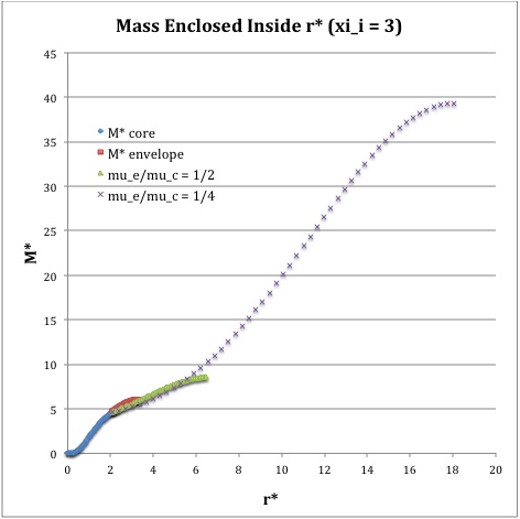
[As of 28 April 2013] For the interface locations <math>\xi_i = 0.5, ~1.0,~\mathrm{and}~3.0</math>, Table 2 provides profiles for three values of the molecular weight ratio: <math>\mu_e/\mu_c = 1.0, ~1/2,~\mathrm{and}~1/4</math>. In all nine graphs, blue diamonds trace the structure of the <math>n_c=5</math> core; the core extends to a radius, <math>r^*_\mathrm{core}</math>, that is independent of molecular weight ratio but varies in direct proportion to the choice of <math>\xi_i</math>. Specifically, as tabulated in the fourth row of Table 1, <math>r^*_\mathrm{core} = 0.34549, ~0.69099, ~\mathrm{and} ~2.07297</math> for, respectively, <math>\xi_i = 0.5,~1,~\mathrm{and}~3</math>. Notice that, while the pressure profile and mass profile are continuous at the interface for all choices of the molecular weight ratio, the density profile exhibits a discontinuous jump that is in direct proportion to the chosen value of <math>\mu_e/\mu_c</math>.
Throughout the <math>n_e = 1</math> envelope, the profile of all physical variables varies with the choice of the molecular weight ratio. In the Table 2 graphs, red squares trace the envelope profile for <math>\mu_e/\mu_c = 1.0</math>; green triangles trace the envelope profile for <math>\mu_e/\mu_c = 1/2</math>; and purple crosses trace the envelope profile for <math>\mu_e/\mu_c = 1/4</math>. The surface of the bipolytropic configuration is defined by the (normalized) radius, <math>R^*</math>, at which the envelope density and pressure drop to zero; the values tabulated in row 16 of Table 1 — <math>1.35550, ~1.62766, ~\mathrm{and} ~3.35697</math> for, respectively, <math>\xi_i = 0.5,~1,~\mathrm{and}~3</math> — correspond to a molecular weight ratio of unity and, hence also, to the envelope profiles traced by red squares in the Table 2 graphs. As the molecular weight ratio is decreased from unity to <math>1/2</math> and, then, <math>1/4</math> for a given choice of <math>\xi_i</math>, the (normalized) radius of the bipolytrope increases roughly in inverse proportion to <math>\mu_e/\mu_c</math> as suggested by the formula for <math>R^*</math> shown in Table 1. This proportional relation is not exact, however, because the parameter <math>\eta_s</math>, which also appears in the formula for <math>R^*</math>, contains an implicit dependence on the chosen value of the molecular weight ratio through the parameter <math>\eta_i</math>.
For a given choice of the interface parameter, <math>\xi_i</math>, the (normalized) mass that is contained in the core is independent of the choice of the molecular weight ratio. However, the (normalized) total mass, <math>M_\mathrm{tot}^*</math>, varies significantly with the choice of <math>\mu_e/\mu_c</math>; as suggested by the expression provided in row 17 of Table 1, the variation is in rough proportion to <math>(\mu_e/\mu_c)^{-2}</math> but, as with <math>R^*</math>, this proportional relation is not exact because the parameters <math>\eta_s</math> and <math>A</math> which also appear in the formula for <math>M_\mathrm{tot}^*</math> harbor an implicit dependence on the molecular weight ratio.
Model Sequences
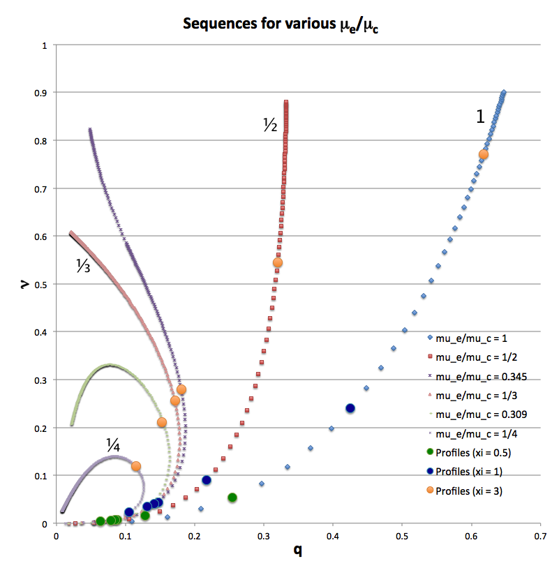
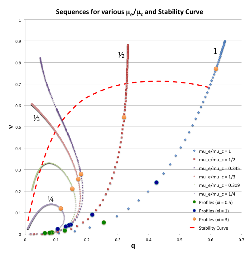
For a given choice of <math>~\mu_e/\mu_c</math> a physically relevant sequence of models can be constructed by steadily increasing the value of <math>\xi_i</math> from zero to infinity — or at least to some value, <math>\xi_i \gg 1</math>. Figure 1 shows how the fractional core mass, <math>\nu \equiv M_\mathrm{core}/M_\mathrm{tot}</math>, varies with the fractional core radius, <math>q \equiv r_\mathrm{core}/R</math>, along sequences having six different values of <math>~\mu_e/\mu_c</math>, as detailed in the figure caption. The natural expectation is that an increase in <math>\xi_i</math> along a given sequence will correspond to an increase in the relative size — both the radius and the mass — of the core. This expectation is realized along the sequences marked by blue diamonds (<math>~\mu_e/\mu_c = 1</math>) and by red squares (<math>~\mu_e/\mu_c = </math>½). But the behavior is different along the other four illustrated sequences. For sufficiently large <math>~\xi_i</math>, the relative radius of the core begins to decrease; then, as <math>~\xi_i</math> is pushed to even larger values, eventually the relative core mass begins to decrease.
|
Figure 1: Analytically determined plot of fractional core mass (<math>~\nu</math>) versus fractional core radius (<math>~q</math>) for <math>~(n_c, n_e) = (5, 1)</math> bipolytrope model sequences having six different values of <math>~\mu_e/\mu_c</math>: 1 (blue diamonds), ½ (red squares), 0.345 (dark purple crosses), ⅓ (pink triangles), 0.309 (light green dashes), and ¼ (purple asterisks). Along each of the model sequences, points marked by solid-colored circles correspond to models whose interface parameter, <math>~\xi_i</math>, has one of three values: 0.5 (green circles), 1 (dark blue circles), or 3 (orange circles); the images linked to Table 2 provide plots of the density, pressure and mass profiles for nine of these identified models. |
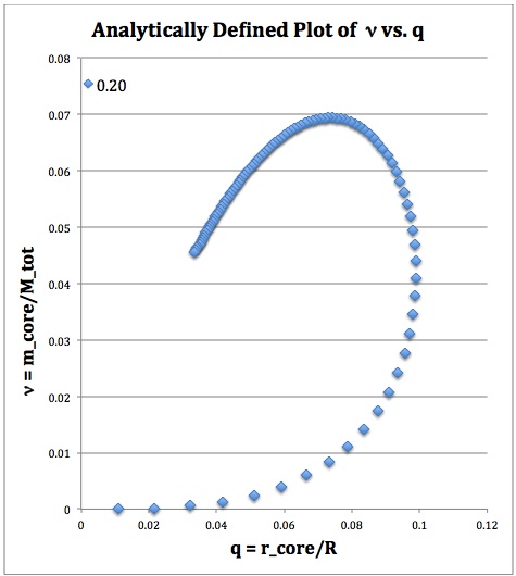
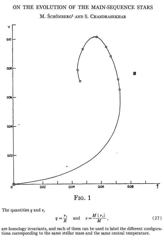
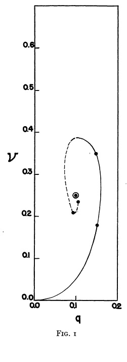
The variation of <math>~\nu</math> with <math>~q</math> for a seventh analytically determined model sequence — one for which <math>~\mu_e/\mu_c = 1/5</math> — is mapped out by a string of blue diamond symbols in the left-hand side of Figure 2. It behaves in an analogous fashion to the <math>~\mu_e/\mu_c = </math>¼ (purple asterisks) sequence displayed in Figure 1. It also quantitatively, as well as qualitatively, resembles the sequence that was numerically constructed by Schönberg & Chandrasekhar (1942) for models with an isothermal core (<math>n_c = \infty</math>) and an <math>~n_e=3/2</math> envelope; Fig. 1 from their paper has been reproduced here on the right-hand side of Figure 2.
|
Figure 2: Relationship to Schönberg-Chandrasekhar Mass Limit |
||
|
Analytic BiPolytrope with <math>n_c=5</math>, <math>n_e = 1</math>, and <math>\mu_e/\mu_c = 1/5</math> |
Edited excerpt from Schönberg & Chandrasekhar (1942) |
Figure from Henrich & Chandraskhar (1941) |
|
(Above) Plot of fractional core mass (<math>\nu</math>) versus fractional core radius (<math>q</math>) for the analytic bipolytrope having <math>\mu_e/\mu_c = 1/5</math>. The behavior of this analytically defined model sequence resembles the behavior of the numerically constructed isothermal core models presented by (center) Schönberg & Chandrasekhar (1942) and by (far right) Henrich & Chandraskhar (1941). |
||
Limiting Mass
Background
As early as 1941, Chandraskhar and his collaborators realized that the shape of the model sequence in a <math>\nu</math> versus <math>q</math> diagram, as displayed in Figure 2 above, implies that equilibrium structures can exist only if the fractional core mass lies below some limiting value. This realization is documented, for example, by the following excerpt from §5 of Henrich & Chandraskhar (1941).
|
Text excerpt from Henrich & Chandraskhar (1941) |
|
Given that our bipolytropic sequence has been defined analytically, it may be possible to analytically determine the limiting core mass of our model. In order to accomplish this, we need to identify the point along the sequence — in particular, the value of the dimensionless interface location — at which <math>d\nu/dq = 0</math> or, equivalently, <math>d\nu/d\xi_i = 0</math>.
Before carrying out the desired differentiations, we will find it useful to rewrite the relevant expressions in terms of the parameters,
<math> \ell_i \equiv \frac{\xi_i}{\sqrt{3}} \, ; </math> and <math> m_3 \equiv 3 \biggl( \frac{\mu_e}{\mu_c} \biggr) \, . </math>
We obtain,
|
<math>\eta_i</math> |
<math>=</math> |
<math>m_3 \biggl( \frac{\ell_i}{1 + \ell_i^2} \biggr) \, ;</math> |
|
<math>\Lambda_i </math> |
<math>=</math> |
<math> \frac{1}{m_3\ell_i} [ 1 + (1-m_3)\ell_i^2] ~~~ \Rightarrow ~~~ </math> Believe it or not … <math> (1 + \Lambda^2) = \frac{(1+\ell_i^2)}{m_3^2 \ell_i^2} \biggl[ 1 + (1-m_3)^2 \ell_i^2 \biggr] \, ; </math> |
|
<math>A</math> |
<math>=</math> |
<math>\biggl[ \frac{1 + (1-m_3)^2 \ell_i^2}{1 + \ell_i^2} \biggr]^{1/2} \, ;</math> |
|
<math>\biggl( \frac{\pi}{2} \biggr)^{1/2} \frac{M_\mathrm{core}}{9}</math> |
<math>=</math> |
<math>\frac{\ell_i^3}{(1 + \ell_i^2)^{3/2}} \, ;</math> |
|
<math>\biggl( \frac{\pi}{2} \biggr)^{1/2} \frac{M_\mathrm{tot}}{9}</math> |
<math>=</math> |
<math> \frac{1}{m_3^2} \biggl[ 1 + (1-m_3)^2 \ell_i^2 \biggr]^{1/2} \biggl\{ \biggl(\frac{\pi}{2} + \tan^{-1} \Lambda_i \biggr) + m_3 \ell_i (1 + \ell_i^2)^{-1} \biggr\} \, . </math> |
Hence,
<math> \nu \equiv \frac{M_\mathrm{core}}{M_\mathrm{tot}} = (m_3^2 \ell_i^3) (1 + \ell_i^2)^{-1/2} [1 + (1-m_3)^2 \ell_i^2]^{-1/2} \biggl[ m_3\ell_i + (1+\ell_i^2) \biggl(\frac{\pi}{2} + \tan^{-1} \Lambda_i \biggr) \biggr]^{-1} </math>
The condition, <math>d\nu/d\xi_i = 0</math>, also will be satisfied if the condition,
<math> \frac{d\ln\nu}{d\ln\ell_i} = 0 \, , </math>
is met.
Derivation
My manual derivation gives,
|
<math> (1+\ell_i^2) \biggl[ \frac{\pi}{2} + \tan^{-1} \Lambda_i \biggr] \biggl\{ 3 - \frac{(1-m_3)^2 \ell_i^2 (1+\ell_i^2)}{[ 1 + (1-m_3)^2 \ell_i^2 ]} \biggr\} </math> |
<math>=</math> |
<math> (1+\ell_i^2) \frac{\partial \tan^{-1}\Lambda_i}{\partial \ln \ell_i} -m_3\ell_i \biggl\{ \ell_i^2 + 2 - \frac{(1-m_3)^2 \ell_i^2 (1+\ell_i^2)}{[ 1 + (1-m_3)^2 \ell_i^2 ]} \biggr\} </math> |
where,
<math> \frac{\partial \tan^{-1}\Lambda_i}{\partial \ln \ell_i} = \frac{[(1-m_3)\ell_i^2 - 1 ] }{m_3\ell_i (1 + \Lambda_i^2)} = \frac{m_3 \ell_i [(1-m_3)\ell_i^2 - 1 ]}{(1 + \ell_i^2) [ 1 + (1-m_3)^2 \ell_i^2]} \, . </math>
Upon rearrangement, this gives,
|
<math> (1+\ell_i^2) \biggl[ \frac{\pi}{2} + \tan^{-1} \Lambda_i \biggr] \biggl\{ 3[ 1 + (1-m_3)^2 \ell_i^2 ] - (1-m_3)^2 \ell_i^2 (1+\ell_i^2) \biggr\} </math> |
<math>=</math> |
<math> m_3\ell_i \biggl\{[(1-m_3)\ell_i^2 - 1 ] -(\ell_i^2 + 2)[ 1 + (1-m_3)^2 \ell_i^2 ] + (1-m_3)^2 \ell_i^2 (1+\ell_i^2) \biggr\} \, ,
</math> |
and further simplification [completed on 19 May 2013] gives,
|
<math> \biggl(\frac{\pi}{2} + \tan^{-1} \Lambda_i\biggr) (1+\ell_i^2) [ 3 + (1-m_3)^2(2-\ell_i^2)\ell_i^2] </math> |
<math>=</math> |
<math> m_3 \ell_i [(1-m_3)\ell_i^4 - (m_3^2 - m_3 +2)\ell_i^2 - 3] \, . </math> |
Limit when <math>m_3 = 0</math>
It is instructive to examine the root of this equation in the limit where <math>m_3 = 0</math> — that is, when <math>\mu_e/\mu_c = 0</math>. First, we note that,
<math>\Lambda_i\biggr|_{m_3 \rightarrow 0} = \biggl\{ \frac{1}{m_3\ell_i} [ 1 + (1-m_3)\ell_i^2] \biggr\}_{m_3 \rightarrow 0} = \infty \, .</math>
Hence,
<math>\biggl[\tan^{-1}\Lambda_i\biggr]_{m_3 \rightarrow 0} = \frac{\pi}{2} \, ,</math>
and the limiting relation becomes,
<math> \pi (1+\ell_i^2) [ 3 + (2-\ell_i^2)\ell_i^2] = 0 \, , </math>
or, more simply,
<math> \ell_i^4 - 2\ell_i^2 - 3 = 0 \, . </math>
The real root is,
<math>\ell_i^2 = \frac{1}{2} \biggl[ 2 + \sqrt{4 + 12} \biggr] = 3 ~~~~ \Rightarrow ~~~~ \xi_i = 3 \, .</math>
For <math>\xi_i = 3</math>, the radius of the core, the mass of the core, and the pressure at the edge of the core are, respectively,
|
<math>r^*_\mathrm{core}</math> |
<math>=</math> |
<math>\biggl(\frac{3^3}{2\pi}\biggr)^{1/2} </math> |
<math>\Rightarrow</math> |
<math>r_\mathrm{core}</math> |
<math>=</math> |
<math>\biggl(\frac{3^3}{2\pi}\biggr)^{1/2} \biggl[ \frac{K_c^{1/2}}{G^{1/2} \rho_0^{2/5}} \biggr] \, ;</math> |
|
<math>M^*_\mathrm{core}</math> |
<math>=</math> |
<math>\biggl(\frac{3^7}{2^5\pi}\biggr)^{1/2} </math> |
<math>\Rightarrow</math> |
<math>M_\mathrm{core}</math> |
<math>=</math> |
<math>\biggl(\frac{3^7}{2^5\pi}\biggr)^{1/2} \biggl[ \frac{K_c^{3/2}}{G^{3/2} \rho_0^{1/5}} \biggr] \, ;</math> |
|
<math>P^*_i</math> |
<math>=</math> |
<math>2^{-6} </math> |
<math>\Rightarrow</math> |
<math>P_i</math> |
<math>=</math> |
<math>2^{-6} [ K_c \rho_0^{6/5}] \, .</math> |
If we invert the middle expression to obtain <math>\rho_0</math> in terms of <math>M_\mathrm{core}</math>, specifically,
<math>\rho_0^{1/5} = \biggl(\frac{3^7}{2^5\pi}\biggr)^{1/2} \biggl[ \frac{K_c^{3/2}}{G^{3/2} M_\mathrm{core}} \biggr] \, ,</math>
then we can rewrite <math>r_\mathrm{core}</math> and <math>P_i</math> in terms of, respectively, the reference radius, <math>R_\mathrm{rf}</math>, and reference pressure, <math>P_\mathrm{rf}</math>, as defined in our discussion of isolated <math>n=5</math> polytropes embedded in an external medium. Specifically, we obtain,
|
<math>r_\mathrm{core}</math> |
<math>=</math> |
<math>\biggl(\frac{3^3}{2\pi}\biggr)^{1/2} \biggl[ \frac{K_c^{1/2}}{G^{1/2} } \biggr] \biggl(\frac{3^7}{2^5\pi}\biggr)^{-1} \biggl[ \frac{K_c^{3/2}}{G^{3/2} M_\mathrm{core}} \biggr]^{-2}</math> |
<math>=</math> |
<math>\biggl(\frac{2^9 \pi}{3^{11}}\biggr)^{1/2} \biggl[ \frac{G^{5/2} M^2_\mathrm{core}}{K_c^{5/2}} \biggr]</math> |
<math>=</math> |
<math>\biggl(\frac{2^9 \pi}{3^{11}}\biggr)^{1/2} \frac{3^3}{2^6} \biggl( \frac{5^5}{\pi} \biggr)^{1/2} R_\mathrm{rf} \biggr|_{n=5}</math> |
<math>=</math> |
<math>\biggl(\frac{5^5}{2^3 \cdot 3^5} \biggr)^{1/2} R_\mathrm{rf} \biggr|_{n=5}</math> |
|
<math>P_i</math> |
<math>=</math> |
<math>2^{-6} [ K_c ] \biggl(\frac{3^7}{2^5\pi}\biggr)^{3} \biggl[ \frac{K_c^{3/2}}{G^{3/2} M_\mathrm{core}} \biggr]^6 </math> |
<math>=</math> |
<math>\biggl(\frac{3^7}{2^{7}\pi}\biggr)^{3} \biggl[ \frac{K_c^{10}}{G^{9} M^6_\mathrm{core}} \biggr] </math> |
<math>=</math> |
<math>\biggl(\frac{3^7}{2^7\pi}\biggr)^{3} \biggl( \frac{2^{26} \pi^3}{3^{12} 5^9} \biggr) P_\mathrm{rf} \biggr|_{n=5}</math> |
<math>=</math> |
<math>\biggl( \frac{2^{5}\cdot 3^9 }{5^9} \biggr) P_\mathrm{rf} \biggr|_{n=5}</math> |
[26 May 2013 with further elaboration on 28 May 2013] This is the same result that was obtained when we embedded an isolated <math>n=5</math> polytrope in an external medium. It shows that the physics that leads to the mass limit for a Bonnor-Ebert sphere is the same physics that sets the Schönberg & Chandrasekhar (1942) mass limit.
Derivation by Eggleton, Faulkner, and Cannon (1998)
The analytically prescribable sequence of bipolytropic models having <math>(n_c, n_e) = (5, 1)</math> displays an interesting behavior that extends beyond identification of a Schönberg-Chandrasekhar-like mass limit. After reaching a maximum value of <math>q</math> but before reaching the maximum value of <math>\nu</math>, the sequence bends back on itself. This means that, even though the fraction of mass enclosed in the core is steadily increasing, the total radius of the configuration is increasing faster than the radius of the core. Qualitatively, at least, this mimics the behavior exhibited by normal stars as they evolve off the main sequence and up the red giant branch.
As I pondered whether or not to probe this analogy in more depth, I recalled — even dating back to my years as a graduate student at Lick Observatory — hearing John Faulkner profess that he finally understood why stars become red giants. I also recalled the following passage from Hansen & Kawaler's (1994) textbook on Stellar Interiors:
|
Excerpt from p. 55 of Hansen & Kawaler (1994) |
|---|
|
The enormous increase in radius that accompanies hydrogen exhaustion moves the star into the red giant region of the H-R diagram. While the transition to red giant dimensions is a fundamental result of all evolutionary calculations, a convincing yet intuitively satisfactory explanation of this dramatic transformation has not been formulated. Our discussion of this phenomenon follows that of Iben and Renzini (1984) although we must state that it is not the whole story.† |
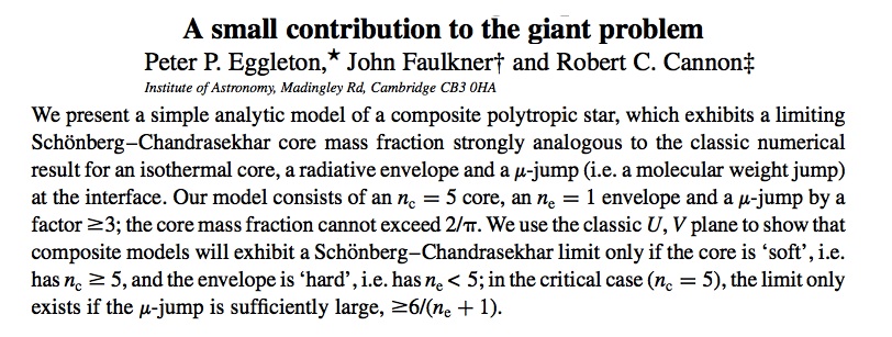
While examining the set of authors who more recently have cited the work by Eggleton & Faulkner (1981), I discovered a paper by Eggleton, Faulkner, and Cannon (1998, MNRAS, 298, 831) with the following title and abstract:
This paper uses analytic techniques to derive precisely the same sequence of <math>~(n_c, n_e) = (5, 1)</math> bipolytropic models that we have presented above.
Free Energy
Here we use this bipolytrope's free energy function to probe the relative dynamical stability of various equilibrium models. This derivation for <math>~(n_c, n_e) = (5, 1)</math> bipolytropes is similar to the one that has been presented elsewhere in the context of <math>~(n_c, n_e) = (0, 0)</math> bipolytropes and follows the analysis outline provided in our discussion of the stability of generalized bipolytropes.
Expression for Free Energy
In order to construct the free energy function, we need mathematical expressions for the gravitational potential energy, <math>~W</math>, and for the thermal energy content, <math>~S</math>, of the models; and it will be natural to break both energy expressions into separate components derived for the <math>~n_c=5</math> core and for the <math>~n_e = 1</math> envelope. Consistent with the above equilibrium model derivations, we will work with dimensionless variables. Specifically, we define,
|
<math>~W^*</math> |
<math>~\equiv</math> |
<math>\frac{W}{[K_c^5/G^3]^{1/2}}</math> |
; |
<math>~S^*</math> |
<math>~\equiv</math> |
<math>\frac{S}{[K_c^5/G^3]^{1/2}} \, .</math> |
Drawing on the various functional expressions that are provided in the above derivations, including the Table of Parameters, integrals over the material in the core give us,
|
<math>~S^*_\mathrm{core}</math> |
<math>~=~</math> |
<math>~ \frac{3}{2} \int_0^{r_i} \biggl(\frac{P^*}{\rho^*}\biggr)_\mathrm{core} (4\pi \rho^*)_\mathrm{core} (r^*)^2 dr^*</math> |
|
|
|
|
<math>~=~</math> |
<math>~ 6\pi \biggl( \frac{3}{2\pi} \biggr)^{3/2} \int_0^{\xi_i} \biggl(1+\frac{1}{3}\xi^2\biggr)^{-3} \xi^2 d\xi</math> |
||
|
|
<math>~=~</math> |
<math>~ 6\pi \biggl( \frac{3^2}{2\pi} \biggr)^{3/2} \int_0^{x_i} \biggl(1+x^2\biggr)^{-3} x^2 dx</math> |
||
|
|
<math>~=~</math> |
<math>~ \biggl( \frac{3^8}{2^7\pi} \biggr)^{1/2} \biggl[ \frac{x_i}{(1+x_i^2)} - \frac{2x_i}{(1+x_i^2)^2} + \tan^{-1}(x_i) \biggr] </math> |
||
|
|
<math>~=~</math> |
<math>~ \frac{1}{2} \biggl( \frac{3^8}{2^5\pi} \biggr)^{1/2} \biggl[ x_i (x_i^4 - 1 )(1+x_i^2)^{-3} + \tan^{-1}(x_i) \biggr] \, ,</math> |
where, in order to streamline the integral for Mathematica, we have used the substitution, <math>~x \equiv \xi/\sqrt{3}</math>; and,
|
<math>~W^*_\mathrm{core}</math> |
<math>~=~</math> |
<math>~ - \int_0^{r_i} (4\pi M_r^* \rho^*)_\mathrm{core} (r^*) dr^*</math> |
|
|
|
|
<math>~=~</math> |
<math>~ - 4\pi \int_0^{\xi_i} \biggl( \frac{2\cdot 3}{\pi } \biggr)^{1/2} \biggl[ \xi^3 \biggl( 1 + \frac{1}{3}\xi^2 \biggr)^{-3/2} \biggr] \biggl( 1 + \frac{1}{3}\xi^2 \biggr)^{-5/2} \biggl( \frac{3}{2\pi} \biggr) \xi d\xi</math> |
||
|
|
<math>~=~</math> |
<math>~ - \biggl( \frac{2^3\cdot 3^8}{\pi } \biggr)^{1/2}\int_0^{x_i} \biggl( 1 + x^2 \biggr)^{-4} x^4 dx</math> |
||
|
|
<math>~=~</math> |
<math>~ - \biggl( \frac{2^3\cdot 3^8}{\pi } \biggr)^{1/2} \biggl[ 3\tan^{-1}(x_i) + \frac{x_i(3x_i^4 -8x_i^2 -3)}{(1+x_i^2)^3} \biggr] \biggl( \frac{1}{2^4 \cdot 3} \biggr) </math> |
||
|
|
<math>~=~</math> |
<math>~ - \biggl( \frac{3^8}{2^5\pi } \biggr)^{1/2} \biggl[ x_i \biggl(x_i^4 - \frac{8}{3} x_i^2 -1 \biggr) (1 + x_i^2)^{-3} + \tan^{-1}(x_i) \biggr] \, .</math> |
(Apology: The parameter <math>~x_i</math> introduced here is identical to the parameter <math>~\ell_i</math> that was introduced earlier in the context of our discussion of the "Limiting Mass" of these models. Sorry for the unnecessary duplication of parameters and possible confusion!)
|
While our aim, here, has been to determine an expression for the gravitational potential energy of a truncated <math>~n = 5</math> polytropic sphere, our derived expression can also give the gravitational potential of an isolated <math>~n = 5</math> polytrope by evaluating the expression in the limit <math>~x_i \rightarrow \infty</math>. In this limit, the first term inside the square brackets goes to zero, while the second term, <math>\lim_{x_i \to \infty}\tan^{-1}(x_i) = \frac{\pi}{2} \, .</math> We see, therefore, that, <math> W^* \biggr|_\mathrm{tot} = \lim_{x_i \to \infty}W^* = - \biggl( \frac{3^8}{2^5\pi } \biggr)^{1/2}\frac{\pi}{2} = - \biggl( \frac{3^8 \pi}{2^7} \biggr)^{1/2} \, . </math> Taking into account our adopted energy normalization, this can be rewritten with the dimensions of energy as,
where we have elected to write the total gravitational potential energy in terms of the natural scale length for <math>~n = 5</math> polytropes, which, as documented elsewhere, is,
As can be seen from the following, boxed-in equation excerpt, our derived expression for the total gravitational potential energy of an isolated <math>~n=5</math> polytrope exactly matches the result derived by H. A. Buchdahl (1978, Astralian J. Phys., 31, 115). The primary purpose of Buchdahl's short paper was to point out that, despite the fact that its radius extends to infinity, "the gravitational potential energy of [an isolated] polytrope of index 5 is finite."
|
Notice that these two terms combine to give, for the core,
|
<math>~\biggl( 2S + W \biggr)_\mathrm{core}</math> |
<math>~=~</math> |
<math>~ \biggl( \frac{2 \cdot 3^6}{\pi } \biggr)^{1/2} \frac{x_i^3}{(1 + x_i^2)^3} = \biggl( \frac{2}{\pi } \biggr)^{1/2} 3^{3/2} \xi_i^3 \biggl( 1 + \frac{1}{3}\xi_i^2 \biggr)^{-3}\, .</math> |
Similarly, integrals over the material in the envelope give us,
|
<math>~S^*_\mathrm{env}</math> |
<math>~=~</math> |
<math>~ \frac{3}{2} \int_{r_i}^R \biggl(\frac{P^*}{\rho^*}\biggr)_\mathrm{env} (4\pi \rho^*)_\mathrm{env} (r^*)^2 dr^*</math> |
|
|
|
|
<math>~=~</math> |
<math>~ 6\pi \int_{\eta_i}^{\eta_s} [\theta^{6}_i \phi^{2}] \biggl[ \biggl( \frac{\mu_e}{\mu_c} \biggr)^{-1} \theta^{-2}_i (2\pi)^{-1/2} \biggr]^3 \eta^2 d\eta</math> |
||
|
|
<math>~=~</math> |
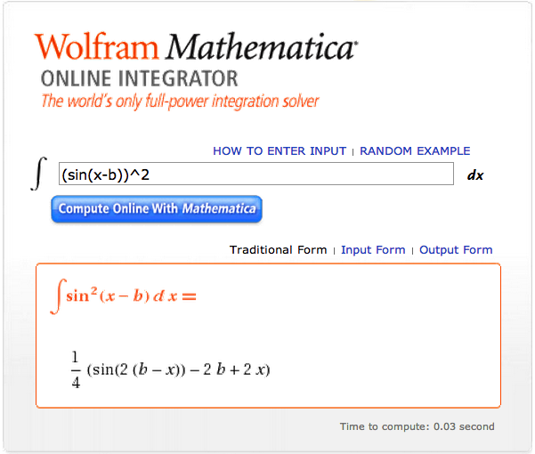
<math>~ \biggl( \frac{3^2}{2\pi} \biggr)^{1/2} \biggl( \frac{\mu_e}{\mu_c} \biggr)^{-3} A^2 \int_{\eta_i}^{\eta_s} [\sin(\eta - B)]^2 d\eta</math> |
||
|
|
<math>~=~</math> |
<math>~ ~ \biggl( \frac{3^2}{2^5\pi} \biggr)^{1/2} \biggl( \frac{\mu_e}{\mu_c} \biggr)^{-3} A^2 \biggl\{ 2(\eta - B) - \sin[2(\eta-B)] \biggr\}_{\eta_i}^{\eta_s} </math> |
||
|
|
<math>~=~</math> |
<math>~ ~ \biggl( \frac{1}{2^5\pi} \biggr)^{1/2} \biggl( \frac{\mu_e}{\mu_c} \biggr)^{-3} A^2 \biggl\{ 6(\eta - B) - 3\sin[2(\eta-B)] \biggr\}_{\eta_i}^{\eta_s} \, ; </math> |
and,
|
<math>~W^*_\mathrm{env}</math> |
<math>~=~</math> |
<math>~ - \int_{r_i}^{R} (4\pi M_r^* \rho^*)_\mathrm{env} (r^*) dr^*</math> |
|
|
|
|
<math>~=~</math> |
<math>~ - 4\pi \int_{\eta_i}^{\eta_s} \biggl( \frac{\mu_e}{\mu_c} \biggr)^{-2} \theta^{-1}_i \biggl( \frac{2}{\pi} \biggr)^{1/2} \biggl(-\eta^2 \frac{d\phi}{d\eta} \biggr) \biggl( \frac{\mu_e}{\mu_c} \biggr) \theta^{5}_i \phi \biggl[ \biggl( \frac{\mu_e}{\mu_c} \biggr)^{-1} \theta^{-2}_i (2\pi)^{-1/2} \biggr]^2 \eta d\eta</math> |
||
|
|
<math>~=~</math> |
<math>~ -\biggl( \frac{2^3}{\pi} \biggr)^{1/2} \biggl( \frac{\mu_e}{\mu_c} \biggr)^{-3} \int_{\eta_i}^{\eta_s} \biggl(-\eta^2 \frac{d\phi}{d\eta} \biggr) \phi \eta d\eta </math> |
||
|
|
<math>~=~</math> |
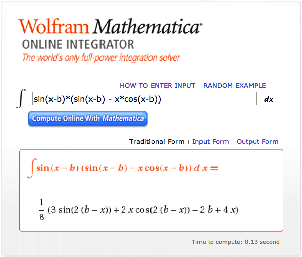
<math>~ -\biggl( \frac{2^3}{\pi} \biggr)^{1/2} \biggl( \frac{\mu_e}{\mu_c} \biggr)^{-3} A^2 \int_{\eta_i}^{\eta_s} [ \sin(\eta-B) - \eta\cos(\eta-B) ] \sin(\eta - B) d\eta </math> |
||
|
|
<math>~=~</math> |
<math>~ -\biggl( \frac{1}{2^3\pi} \biggr)^{1/2} \biggl( \frac{\mu_e}{\mu_c} \biggr)^{-3} A^2 \biggl\{ - 3\sin[2(\eta - B)] +2\eta \cos[2(\eta - B)] + 4(\eta - B) + 2B \biggr\}_{\eta_i}^{\eta_s} </math> |
||
|
|
<math>~=~</math> |
<math>~ -\biggl( \frac{1}{2^3\pi} \biggr)^{1/2} \biggl( \frac{\mu_e}{\mu_c} \biggr)^{-3} A^2 \biggl\{6(\eta-B) - 3\sin[2(\eta - B)] -4\eta\sin^2(\eta-B) + 4B \biggr\}_{\eta_i}^{\eta_s} \, . </math> |
In this case, the two terms combine to give, for the envelope,
|
<math>~\biggl( 2S + W \biggr)_\mathrm{env}</math> |
<math>~=~</math> |
<math>\biggl( \frac{1}{2^3\pi} \biggr)^{1/2} \biggl( \frac{\mu_e}{\mu_c} \biggr)^{-3} A^2 \biggl[4\eta\sin^2(\eta-B) + 4B \biggr]_{\eta_i}^{\eta_s}</math> |
|
|
<math>~=~</math> |
<math>\biggl( \frac{2}{\pi} \biggr)^{1/2} \biggl( \frac{\mu_e}{\mu_c} \biggr)^{-3} A^2 \biggl[\eta_s\sin^2(\eta_s-B) - \eta_i\sin^2(\eta_i-B) \biggr] \, .</math> |
Equilibrium Condition
Recognizing from the above Table of Parameters that,
|
<math>~A</math> |
<math>~=~</math> |
<math>~\frac{\eta_i}{\sin(\eta_i - B)} \, ,</math> |
[because <math>~\phi_i = 1</math>] |
|
<math>~(\eta_s - B)</math> |
<math>~=~</math> |
<math>~\pi \, ,</math> |
[hence, <math>~\sin^2(\eta_s - B) = 0</math>] |
|
<math>~\eta_i</math> |
<math>~=~</math> |
<math>~3^{1/2} \biggl( \frac{\mu_e}{\mu_c} \biggr) \xi_i \biggl( 1 + \frac{1}{3} \xi_i^2 \biggr)^{-1}\, ,</math> |
|
we can rewrite this last "envelope virial" expression as,
|
<math>~\biggl( 2S + W \biggr)_\mathrm{env}</math> |
<math>~=~</math> |
<math>- ~ \biggl( \frac{2}{\pi} \biggr)^{1/2} \biggl( \frac{\mu_e}{\mu_c} \biggr)^{-3} \eta_i^3</math> |
|
|
<math>~=~</math> |
<math>- ~ \biggl( \frac{2}{\pi} \biggr)^{1/2} 3^{3/2} \xi_i^3 \biggl( 1 + \frac{1}{3} \xi_i^2 \biggr)^{-3} \, .</math> |
This expression is equal in magnitude, but opposite in sign to the "core virial" expression derived earlier. Hence, putting the core and envelope contributions together, we find,
|
<math>~\biggl( 2S + W \biggr)_\mathrm{tot} ~=~ 2(S_\mathrm{core} + S_\mathrm{env}) + (W_\mathrm{core} + W_\mathrm{env})</math> |
<math>~=~</math> |
<math>~ 0 \, .</math> |
This demonstrates that the detailed force-balanced models of <math>~(n_c, n_e) = (5,1)</math> bipolytropes derived above are also all in virial equilibrium, as should be the case. More importantly, showing that these four separate energy integrals sum to zero helps provide confirmation that the four energy integrals have been derived correctly. This allows us to confidently proceed to an evaluation of the relative dynamical stability of the models.
Stability Condition
According to the accompanying free-energy based, generalized formulation of stability in bipolytropes, our above derived <math>~(n_c, n_e) = (5,1)</math> bipolytropes — or, equivalently, <math>~(\gamma_c, \gamma_e) = (6/5, 2)</math> bipolytropes — will be dynamically stable only if,
|
<math>~ - (W_\mathrm{core} + W_\mathrm{env}) \biggl( \gamma_e - \frac{4}{3}\biggr) </math> |
<math>~>~</math> |
<math> ~ 2(\gamma_e-\gamma_c) S_\mathrm{core} \, .</math> |
Otherwise, they will be dynamically unstable toward radial perturbations. For various values of the <math>~\mu_e/\mu_c</math> ratio, Table 1 identifies the value of <math>~\xi_i</math> — and the corresponding values of <math>~q</math> and <math>~\nu</math> — at which the left-hand side of this stability relation equals the right-hand side. The locus of points provided by Table 1 defines the curve that separates stable from unstable regions of the <math>~q-\nu</math> parameter space. The red-dashed curve drawn in Figure 3 graphically depicts this demarcation: the region below the curve identifies bipolytrope models that are dynamically stable while the region above the curve identifies unstable models.
|
|||||||||||||||||||||||||||||||||||||||||||||||||||||||||||||||||||||||||||||||||||||||||||||||||||||||||||
|
Figure 3: Largely the same as Figure 1, above, but a red-dashed curve has been added that separates the <math>~q - \nu</math> domain into regions that contain stable models (lying below the curve) from dynamically unstable models (lying above the curve), as determined by the virial stability analysis presented here. |
|||||||||||||||||||||||||||||||||||||||||||||||||||||||||||||||||||||||||||||||||||||||||||||||||||||||||||
Related Discussions
- Polytropes emdeded in an external medium
- Constructing BiPolytropes
- Bonnor-Ebert spheres
- Bonnor-Ebert Mass according to Wikipedia
- A MATLAB script to determine the Bonnor-Ebert Mass coefficient developed by Che-Yu Chen as a graduate student in the University of Maryland Department of Astronomy
- Schönberg-Chandrasekhar limiting mass
- Relationship between Bonnor-Ebert and Schönberg-Chandrasekhar limiting masses

|
|---|
|
© 2014 - 2021 by Joel E. Tohline |
