User:Tohline/SSC/Structure/IsothermalSphere

Isothermal Sphere (structure)

Here we supplement the simplified set of principal governing equations with an isothermal equation of state, that is, <math>~P</math> is related to <math>~\rho</math> through the relation,

<math>P = c_s^2 \rho \, ,</math>

where, <math>c_s</math> is the isothermal sound speed. Comparing this <math>~P</math>-<math>~\rho</math> relationship to

Form A
of the Ideal Gas Equation of State,

<math>~P_\mathrm{gas} = \frac{\Re}{\bar{\mu}} \rho T</math>

we see that,

<math>c_s^2 = \frac{\Re T}{\bar{\mu}} = \frac{k T}{m_u \bar{\mu}} \, ,</math>

where, <math>~\Re</math>, <math>~k</math>, <math>~m_u</math>, and <math>~\bar{\mu}</math> are all defined in the accompanying variables appendix. It will be useful to note that, for an isothermal gas, <math>~H</math> is related to <math>~\rho</math> via the expression,

<math> dH = \frac{dP}{\rho} = c_s^2 d\ln\rho \, . </math>

Governing Relations

Adopting solution technique #2, we need to solve the following second-order ODE relating the two unknown functions, <math>~\rho</math> and <math>~H</math>:

<math>\frac{1}{r^2} \frac{d}{dr}\biggl( r^2 \frac{dH}{dr} \biggr) =- 4\pi G \rho</math> .

Using the <math>~H</math>-<math>~\rho</math> relationship for an isothermal gas presented above, this can be rewritten entirely in terms of the density as,

<math>\frac{1}{r^2} \frac{d}{dr}\biggl( r^2 \frac{d\ln\rho}{dr} \biggr) =- \frac{4\pi G}{c_s^2} \rho \, ,</math>

or, equivalently,

<math> \frac{d^2\ln\rho}{dr^2} +\frac{2}{r} \frac{d\ln\rho}{dr} + \beta^2 \rho = 0 \, , </math>

where,

<math> \beta^2 \equiv \frac{4\pi G}{c_s^2} \, . </math>

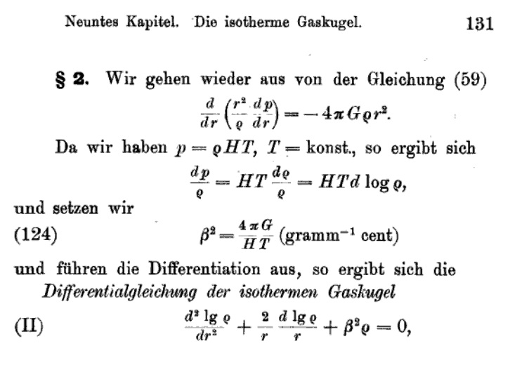
This matches the governing ODE whose derivation was published on p. 131 of Robert Emden's (1907) book titled, Gaskugeln.

Derivation by Emden (edited)

By adopting the following dimensionless variables,

<math> \mathfrak{r}_1 \equiv \rho_c^{1/2} \beta r \, , ~~~~\mathrm{and}~~~~v_1 \equiv \ln(\rho/\rho_c) \, , </math>

where <math>\rho_c</math> is the configuration's central density, the governing ODE can be rewritten in dimensionless form as,

<math> \frac{d^2v_1}{d\mathfrak{r}_1^2} +\frac{2}{\mathfrak{r}_1} \frac{dv_1}{dr} + e^{v_1} = 0 \, , </math>

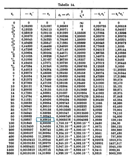
which is exactly the equation numbered (II"a) that can be found on p. 133 of Emden (1907). Emden numerically determined the behavior of the function <math>v_1(\mathfrak{r}_1)</math>, its first derivative with respect to <math>\mathfrak{r}_1</math>, <math>v_1'</math>, along with <math>e^{v_1}</math> and several other useful products, and published his results as Table 14, on p. 135 of his book. The table is reproduced here, primarily for historical purposes.

Emden's Numerical Solution

Note: The entry highlighted in blue in the <math>3^\mathrm{rd}</math> column must be a typesetting error.

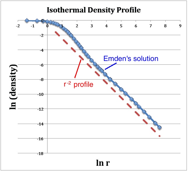
A plot of <math>v_1</math> versus <math>\ln\mathfrak{r}_1</math>, as shown below in Figure 1a, translates into a log-log plot of the equilibrium configuration's <math>\rho(r)</math> density profile.

Figure 1: Emden's Numerical Solution
(a) The <math>(x,y)</math> locations of the data points plotted in blue are drawn directly from column 1 and column 3 of Emden's Table 14 — specifically, <math>x = \ln(\mathfrak{r}_1)</math> and <math>y = v_1</math>. The dashed red line has a slope of <math>-2</math> and serves to illustrate that, at large radii, the isothermal density profile tends toward a <math>\rho \propto r^{-2}</math> distribution.	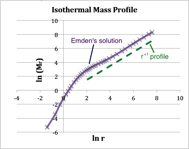(b) The <math>(x,y)</math> locations of the data points plotted in purple are drawn directly from column 1 and column 7 of Emden's Table 14 — specifically, <math>x = \ln(\mathfrak{r}_1)</math> and <math>y = \mathfrak{r}_1^2 v_1'</math>. The dashed green line has a slope of <math>+1</math> and serves to illustrate that, at large radii, the isothermal <math>M(r)</math> distribution tends toward a <math>M_r \propto r</math> distribution.

Bonnor and Ebert

In their studies of pressure-bounded isothermal spheres, Ebert (1955, ZA, 37, 217) and Bonnor (1956, MNRAS, 116, 351) both started with this governing ODE, but developed its solution in different ways. Here we present both developments while highlighting transformations between the two.

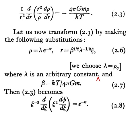
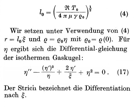
Derivation by Bonnor (edited)	translation	Derivation by Ebert (edited)
	<math>G \Leftrightarrow \gamma</math>
	<math>\rho_c \Leftrightarrow \rho_0</math>
	<math>\frac{kT}{m} \Leftarrow c_s^2 \Rightarrow \frac{\Re T_0}{\mu}</math>
	<math>\beta^{1/2}\lambda^{-1/2} \Leftrightarrow l_0</math>
	<math>e^{-\psi} \Leftrightarrow \eta</math>

Related Wikipedia Discussions

• Isothermal Sphere

© 2014 - 2021 by Joel E. Tohline |   H_Book Home   |   YouTube   | Appendices: | Equations | Variables | References | Ramblings | Images | myphys.lsu | ADS | Recommended citation:   Tohline, Joel E. (2021), The Structure, Stability, & Dynamics of Self-Gravitating Fluids, a (MediaWiki-based) Vistrails.org publication, https://www.vistrails.org/index.php/User:Tohline/citation