User:Tohline/IVAJ/Level1

Most of the content of this Wiki document initially appeared in print as a Visualization Corner article in the May/June 2009 issue of Computing in Science & Engineering.

A Customized Python Module for CFD Flow Analysis within VisTrails
by Joel E. Tohline, Jinghua Ge, Wesley Even, & Erik Anderson

A relatively simple, customized Python module that plugs smoothly into an otherwise standard workflow within VisTrails facilitates a quantitative analysis of complex fluid flows in simulations of merging binary stars.

Introduction

Researchers in the open source community are steadily improving scientific visualization tools. These tools are providing a wider array of sophisticated probes for data analysis and a wider assortment of effective user-friendly interfaces. They're also making it easier for researchers in the computational science community — across many disciplines — to effectively analyze huge datasets by drawing on the human brain's acute ability to sort through complex and time-varying visual patterns. The astrophysics group at Louisiana State University (LSU), for example, routinely uses volume-rendering and ray-tracing algorithms in conjunction with animation techniques to examine the time-varying behavior of isodensity surfaces that arise in computational fluid dynamic (CFD) simulations of mass-transferring and merging binary star systems. Although such analyses generally provide only a qualitative identification and assessment of structure within a given dataset, the insight gained from visual inspection can nevertheless be extremely valuable. For example, it was through visual inspection that researchers at LSU initially spotted the nonlinear development of triangular-, square-, and pentagonal-shaped tidal resonances in recent simulations.

LSU's astrophysics group has begun to incorporate VisTrails into its arsenal of scientific visualization and data analysis tools. VisTrails primarily interested the group a few years ago because it provides a user-friendly workflow interface to the extensive VTK software library. It also automatically tracks the provenance of data analysis efforts. However, what most impresses us now is the ease with which VisTrails facilitates the insertion of home-grown analysis modules into an otherwise VTK-based workflow. Taking advantage of this additional programming versatility, we have gained a greater appreciation of the role that visualization tools can play in the quantitative assessment of results from large-scale simulations. In this article, we first describe the VTK-based workflow that we initially constructed in VisTrails to view streamlines within each binary mass-transfer simulation. We then describe the Python module, whose insertion into this workflow has permitted us to identify values of key rotational frequencies associated with such flows.

Base Workflow

Figure 1: (scroll over image for caption)

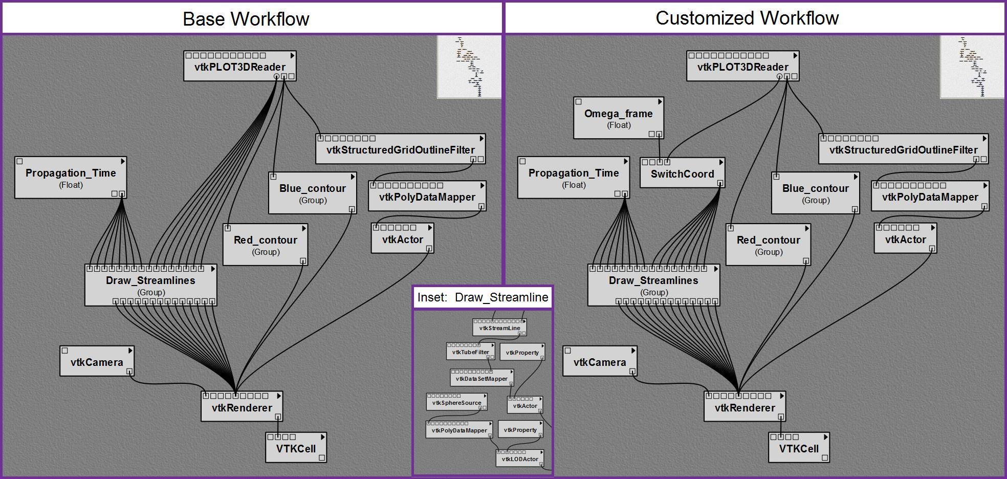
Within VisTrails, we initially selected various VTK-based modules to do the following, in sequence (see Figure 1a):

• Read simulation data. We used vtkPLOT3DReader to read in one file containing the <math>(x, y, z)</math> coordinate locations of every vertex on our 3D cylindrical coordinate mesh and a separate file containing the fluid's mass-density (scalar) and momentum-density (3D vector) at every grid vertex.
• Outline cylindrical domain boundary. As shown, we enlisted vtkStructuredGridOutlineFilter, vtkPolyDataMapper, and vtkActor.
• Define isodensity surfaces. We rendered two nested isodensity surfaces to outline high- (red) and low-density (blue) flow regions. The Red_contour and Blue_contour module groups each contain vtkContourFilter, vtkDataSetMapper, vtkProperty, and vtkActor.
• Draw streamlines. As Figure 1b shows, each of the eight separate Draw_Streamlines module groups uses vtkStreamLine, vtkTubeFilter, vtkDataSetMapper, vtkProperty, vtkActor, vtkSphereSource, vtkPolyDataMapper, and vtkLODActor to trace an individual streamline within the flow. Streamline lengths are set by feeding a common Propagation_Time into all eight module groups.

Vistrails renders the output from the various workflow actors in a composite scene using vtkRenderer as viewed by an observer located at a position that vtkCamera specifies. Finally, the module vtkCell directs this scene to the VisTrails interactive spreadsheet.

In this initially constructed base workflow, VisTrails pipes the 3D vector field representing the momentum density distribution from the vtkPLOT3DReader module directly into each of the eight Draw_Streamline module groups. This base workflow — which VisTrails assembles using generically available vtk modules — lets us examine the behavior of streamlines in our binary mass-transfer simulations, but only from the frame of reference, <math>\Omega_0</math>, in which we originally performed each simulation (see Figure 2b, labeled <math>\Delta\Omega = 0.00</math>).

TERMINOLOGY One well-defined characteristic of a binary star system is it orbital period, <math>P</math>. If the stars are in circular orbit around one another, a binary system will appear to be stationary when viewed from a frame that's rotating with an angular frequency <math>\Omega_\mathrm{frame} = 2\pi/P</math>. When modeling mass-transferring binary star systems, we've found it advantageous to perform each computational fluid dynamic (CFD) simulation on a cylindrical-coordinate grid that rotates with a frequency <math>\Omega_0 = 2\pi/P_0</math>, where <math>P_0</math> is the binary system's orbital period at the beginning of the simulation. As mass and angular momentum are transferred from one star to the other throughout the simulation, however, the binary system's orbital period &#150; and associated value of <math>\Omega_\mathrm{frame}</math> &#150; will vary. As explained in the main text, we used VisTrails to measure <math>\Delta\Omega = (\Omega_\mathrm{frame} - \Omega_0)</math> and, hence, the instantaneous orbital period <math>P = P_0/(1 + P_0 \Delta\Omega/2\pi)</math> at any time during a simulation.

Customized Python Module

To make it possible for us to examine the properties of binary mass-transfer flows from reference frames that have a range of different angular frequencies of rotation, <math>\Omega_\mathrm{frame} = (\Omega_0 + \Delta\Omega)</math>, we wrote a Python-based module &#150; SwitchCoord &#150; for insertion into the base VisTrails workflow. Figure 1c shows our resulting customized VisTrails workflow; it differs very little from the base workflow. The sidebar shows the complete Python source code from our customized module. The code segment that performs the required physics analysis is short and straightforward. In particular, the SwitchCoord module performs the following operations at each grid vertex:

• converts the <math>(x, y)</math> Cartesian to <math>(R, \phi)</math> cylindrical coordinates;
• divides the momentum components by density to obtain the velocity components if the density is greater than minp (otherwise, it sets the velocity components to zero);
• shifts the azimuthal velocity component <math>v_\phi</math> to a new, rotating frame of reference by adding <math>R\times \Delta\Omega</math>;
• converts the cylindrical velocity components to Cartesian velocity components; and
• normalizes the velocities to the maximum velocity maxnorm found across the domain where densities are greater than minp.

We designed the output ports on SwitchCoord to provide access to the same type of structured arrays that vtkPLOT3DReader generates. But, in our customized VisTrails workflow, which includes SwitchCoord (see Figure 1c), the 3D vector field that VisTrails pipes into each of the eight Draw_Streamline module groups represents the fluid's velocity distribution as viewed from the rotating frame of reference that the floating-point scalar, Omega_frame, specifies.

Interpretation of Results

Figure 2 (scroll over image for caption)

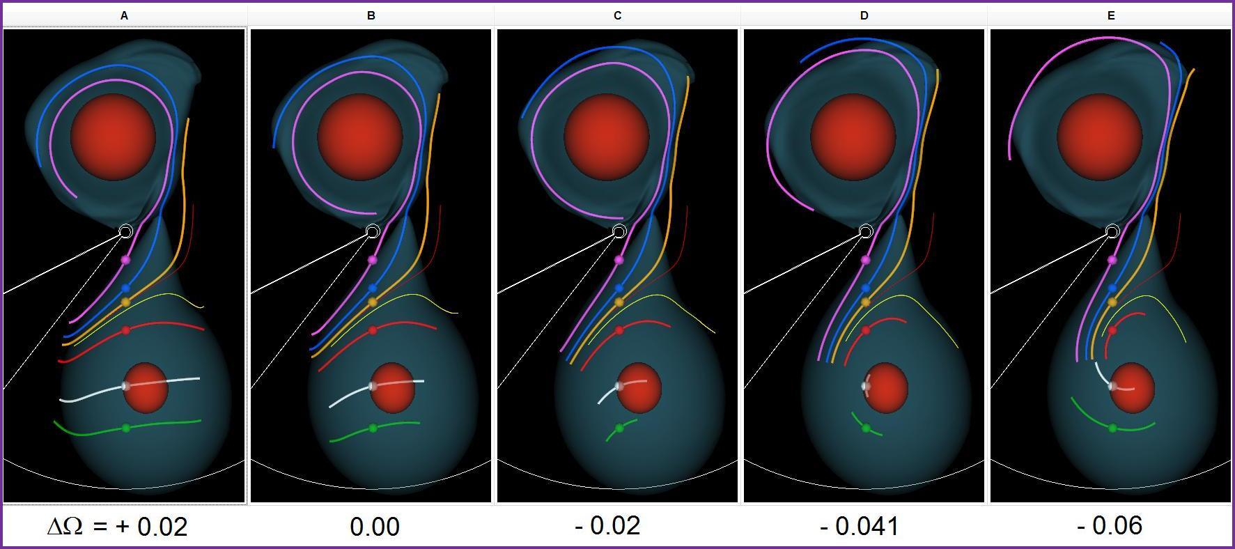
Figure 2 displays 3D renderings of the flow from one of our binary mass-transfer simulations as generated by our customized VisTrails workflow. We have generated images assuming five different frame rotation frequencies, as specified by <math>\Delta\Omega</math>. Aside from labeling <math>\Delta\Omega</math> values under each image, we produced Figure 2 by simply taking a screenshot of the VisTrails interactive spreadsheet. The spreadsheet feature has proven to be extremely useful in this analysis because it facilitates the side-by-side comparison of scenes that VisTrails has rendered using different parameter values. And, although we can't demonstrate it here in print, VisTrails lets users zoom, pan, and interactively rotate all 3D-rendered scenes simultaneously.

We'd like to determine which value of <math>\Delta\Omega</math> provides the best measure of the binary star system's true orbital period. As expected, for all five choices of <math>\Delta\Omega</math>, we found the highest velocities (marked by the longest streamlines) along the relatively low-density mass-transfer stream that connects the two stars. Material from the donor star (in the lower half of each rendered image in Figure 2) flows toward its stellar companion, reaching supersonic velocities before impacting the companion. An oblique shock front &#150; whose location is delineated by kinks in the pink, blue, and orange streamlines &#150; terminates the component of motion perpendicular to the companion's surface. Motion transverse to the shock becomes orbital motion in a thick, low-density disk that surrounds the companion star.

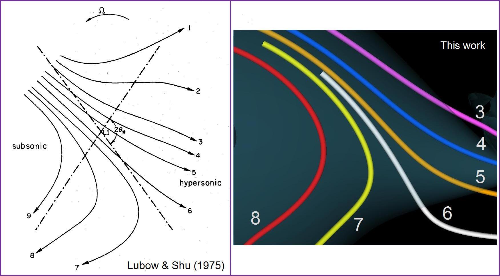
For all five choices of <math>\Delta\Omega</math>, the flow's behavior in the vicinity of the mass-transfer stream very closely resembles the behavior that Stephen Lubow and Frank Shu predicted more than 30 years ago. Figure 3b shows the magnified view of this region of the flow from our simulation assuming <math>\Delta\Omega = - 0.041</math>. We've reoriented this magnified image and numbered the streamlines to facilitate comparison with the Lubow and Shu illustration, which we've reprinted with permission here (see Figure 3a). Rather than conducting a fully self-consistent 3D simulation &#150; which was computationally impractical at the time &#150; Lubow and Shu used a mathematical perturbation analysis to estimate what the flow should look like in the vicinity of the "L1" Lagrange point, as viewed from a frame of reference rotating with the correct instantaneous orbital frequency, <math>\Omega_\mathrm{frame}</math>. The close resemblance between our 3D simulation results in the vicinity of the L1 Lagrange point, and the behavior that Lubow and Shu predicted provides a useful point of verification for our work.

Each star's center of mass should lie near the center of the highest density region inside each star (outlined by the nearly spherical, red isodensity surfaces in Figure 2). When we've assigned <math>\Delta\Omega</math> a value that properly identifies the frequency at which the centers of mass of the two stars are orbiting one another, we should see very little residual motion near the donor star's center &#150; that is, streamlines rendered in white and green in Figure 2 should be quite short. Furthermore, we expect that this residual motion should translate into concave streamline segments, mapping out simple circular motion around the center of the donor star. When we've identified the correct value of <math>\Delta\Omega</math>, we also should expect the returning streamline nearest the mass-transfer stream (colored yellow) to remain inside the donor. With these ideas in mind, we judge <math>\Delta\Omega = - 0.041</math>.

Finally, we note that as the pink and blue streamlines curve around the companion star, they extend outside the companion's disk (as outlined by the blue isodensity surface) in the rendered images with the most negative specified values of <math>\Delta\Omega</math>. These two streamlines appear to align most neatly with the distribution of material in the disk in Figure 2a, that is, for <math>\Delta\Omega = + 0.02</math>. This suggests that there's a characteristic frequency associated with motion in the companion's disk that's different from the binary orbital frequency.

Figure 3 (scroll over image for caption)

Summary

We've illustrated how, at one particular instant during a CFD simulation, we can determine the orbital period of our simulated binary star system. With this customized visualization tool in hand, we're in a position to determine how the orbital period and other characteristic frequencies vary with time throughout each simulation. More significantly, we now appreciate how we can modify otherwise standard VisTrails workflows to perform any of a variety of analysis tasks that are customized to our research project needs.

Addenda

Acknowledgments

Progress on this project has benefitted significantly from interactions with Claudio Silva, Juhan Frank, Patrick Motl, and Zach Byerly. This work has been supported, in part, by funding from the US National Science Foundation (AST-0708551, DGE-0504507), the US Department of Energy, NASA (ATP-NNX07AG84G), and IBM; mass-transfer simulations were made possible via allocations of computing time on TeraGrid resources (TG-MCA98N043) at the National Center for Supercomputer Applications (NCSA) and through the Louisiana Optical Network Initiative (LONI).

References

1. J.E. Tohline, "Scientific Visualization: A Necessary Chore," Computing in Science & Eng., vol. 9, no. 6, 2007, pp. 76-81.
2. M.C.R. D'Souza et al., "Numerical Simulations of the Onset and Stability of Dynamical Mass Transfer in Binaries," Astrophysical J., vol. 643, no. 1, 2006, pp. 381-401.
3. P.M. Motl, et al., "The Stability of Double White Dwarf Binaries Undergoing Direct Impact Accretion," Astrophysical J., vol. 670, no. 1, 2007, pp. 1314-1325.
4. L. Bavoil et al., "Vistrails: Enabling Interactive Multiple-View Visualizations," 2005; www.sci.utah.edu/~csilva/papers/vis2005b.pdf.
5. S.H. Lubow and F.H. Shu, "Gas Dynamics of Semidetached Binaries," Astrophysical J., vol. 198, no. 1, 1975, pp.383-405.

About the Authors

• Joel E. Tohline is a professor at Louisiana State University. His research interests include astrophysics, computational fluid dynamics, and high-performance computing. Tohline has a PhD in astronomy from the University of California, Santa Cruz. He's a fellow of the American Association for the Advancement of Science, and a member of the International Astronomical Union, the American Astronomical Society, and the American Physical Society. Contact him at tohline@lsu.edu.
• Jinghua Ge is a visualization consultant at the Center for Computation & Technology (CCT) at Louisiana State University. Her research interests include scientific visualization, computer graphics, and distributed computing. Ge has a PhD in computer science from the University of Illinois, Chicago. Contact her at jinghuage@cct.lsu.edu.
• Wesley Even is an NSF/IGERT fellow in the Department of Physics and Astronomy at Louisiana State University. His research focuses on the modeling of mass transfer in double-white-dwarf binary star systems. Contact him at weseven@physics.lsu.edu.
• Erik Anderson is a research assistant and PhD candidate at the University of Utah. His research interests include scientific visualization, signal processing, computer graphics, and multimodal visualization. Anderson has a BS in computer science and a BS in electrical and computer engineering from Northeastern University. Contact him at eranders@sci.utah.edu.

---

---

Sidebar: SwithCoord Python Module

Here we present a complete listing of the python code from our customized SwitchCoord program module. At the beginning of the "Physics Analysis" segment of the code, we assign names to the data arrays that have been acquired as input from vtkPLOT3DReader: pcoords is a tuple that identifies the Cartesian-based coordinate location of each grid vertex, density is a scalar that specifies the mass density, and momentum is a tuple that specifies the values of the cylindrical-coordinate-based vector momentum at each grid vertex. We detail the remaining logic of the physics analysis in the main text.

import core.modules.module_registry
from core.modules.vistrails_module import Module, ModuleError
import vtk, math
version="0.0.0"
name="SwitchCoord"
identifier="edu.lsu.switchcoord"

class SwitchCoord(Module):
    def compute(self):
        minp = self.getInputFromPort("min_density")
        Domega = self.getInputFromPort("Domega")
        dataset=self.getInputFromPort("dataset")
        output = self.create_instance_of_type('edu.utah.sci.vistrails.vtk', 'vtkStructuredGrid')
        output.vtkInstance = vtk.vtkStructuredGrid()
        mydata=output.vtkInstance
        mydata.DeepCopy(dataset.vtkInstance)
        self.op(mydata, minp, omega)
        self.setResult("changed_dataset", output)

    ###################################
    ##
    ## Begin:  Physics Analysis
    ##
    ###################################

    def op(self, mydata, minp, omega):
        extent=mydata.GetExtent()
        pcoords = mydata.GetPoints().GetData()
        density = mydata.GetPointData().GetScalars("Density")
        momentum = mydata.GetPointData().GetVectors("Momentum")

        maxnorm = 0.0
        for i in range(0, mydata.GetNumberOfPoints()):
            [x, y, z] = pcoords.GetTuple3(i)  
            [_v1, _v2, _v3] = momentum.GetTuple3(i)
            p = density.GetValue(i)
            r = math.sqrt(x*x + y*y)         
            phi = math.atan2(y, x)
            if p < minp: 
                vx=vy=vz=0
            else:
                vr = _v1 / p
                vphi = _v2 / (p) + r * omega
                vz = _v3 / p
                vx = vr * math.cos(phi) - vphi * math.sin(phi)
                vy = vr * math.sin(phi) + vphi * math.cos(phi)

                norm = math.sqrt(vx*vx + vy*vy + vz*vz)
                if norm > maxnorm:
                    maxnorm = norm
            momentum.SetTuple3(i, vx, vy, vz)

        for i in range(0, mydata.GetNumberOfPoints()):
            [vx, vy, vz] = momentum.GetTuple3(i)
            vx = vx/maxnorm
            vy = vy/maxnorm
            vz = vz/maxnorm
            momentum.SetTuple3(i, vx, vy, vz)

    ###################################
    ##
    ## End:  Physics Analysis
    ##
    ###################################

def initialize(*args, **keywords):
    reg=core.modules.module_registry.registry
    reg.add_module(SwitchCoord)
    reg.add_input_port(SwitchCoord, "scalar_range", 
                       [core.modules.basic_modules.Float, 
                        core.modules.basic_modules.Float]) 
    reg.add_input_port(SwitchCoord, "min_density", core.modules.basic_modules.Float)
    reg.add_input_port(SwitchCoord, "omega", core.modules.basic_modules.Float)
    reg.add_input_port(SwitchCoord, "dataset", 
                       (reg.get_descriptor_by_name(
                'edu.utah.sci.vistrails.vtk', 'vtkStructuredGrid').module) )
    reg.add_output_port(SwitchCoord, "changed_dataset", 
                        (reg.get_descriptor_by_name(
                'edu.utah.sci.vistrails.vtk', 'vtkStructuredGrid').module) )

def package_dependencies():
    import core.packagemanager
    manager = core.packagemanager.get_package_manager()
    if manager.has_package('edu.utah.sci.vistrails.vtk'):
        return ['edu.utah.sci.vistrails.vtk']
    else:
        return []