Difference between revisions of "User:Tohline/Appendix/Ramblings/RiemannB74C692"
| Line 21: | Line 21: | ||
</td> | </td> | ||
<td align="center" colspan="3"> | <td align="center" colspan="3"> | ||
<math>~\frac{b}{a} = 0. | <math>~\frac{b}{a} = 0.74</math> | ||
</td> | </td> | ||
<td align="center" rowspan="5" width="2%"> | <td align="center" rowspan="5" width="2%"> | ||
| Line 34: | Line 34: | ||
<tr> | <tr> | ||
<td align="center" colspan="3"> | <td align="center" colspan="3"> | ||
<math>~\frac{c}{a} = 0. | <math>~\frac{c}{a} = 0.692</math> | ||
</td> | </td> | ||
</tr> | </tr> | ||
| Line 52: | Line 52: | ||
<tr> | <tr> | ||
<td align="center"> | <td align="center"> | ||
<math>~\Omega_\mathrm{EFE} = 0. | <math>~\Omega_\mathrm{EFE} = 0.638747</math> | ||
</td> | </td> | ||
<td align="center"> | <td align="center"> | ||
<math>~\Omega_\mathrm{EFE} = - 0. | <math>~\Omega_\mathrm{EFE} = - 0.217773</math> | ||
</td> | </td> | ||
</tr> | </tr> | ||
| Line 61: | Line 61: | ||
<tr> | <tr> | ||
<td align="center"> | <td align="center"> | ||
<math>~\lambda_\mathrm{EFE} = 0. | <math>~\lambda_\mathrm{EFE} = 0.217773</math> | ||
</td> | </td> | ||
<td align="center"> | <td align="center"> | ||
<math>~\lambda_\mathrm{EFE} = - 0. | <math>~\lambda_\mathrm{EFE} = - 0.638747 </math> | ||
</td> | </td> | ||
</tr> | </tr> | ||
Revision as of 02:53, 29 May 2020
Another S-type Example b74c692
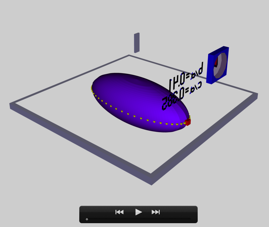
This chapter is an extension of the chapter we have titled, "Riemann Meets COLLADA & Oculus Rift S." In that chapter we used as our first example of a Riemann S-type ellipsoid the model with parameters, b41c385. Other closely related chapters are listed below under the heading, "See Also".

|
|---|
| | Tiled Menu | Tables of Content | Banner Video | Tohline Home Page | |
Key Physical Parameters
The model that we have chosen to use in our second successful construction of a COLLADA-based, 3D and interactive animation has the following properties; this model has been selected from Table 2 of our accompanying discussion of Riemann S-type ellipsoids:
|
|
<math>~\frac{b}{a} = 0.74</math> |
|
||||
|
<math>~\frac{c}{a} = 0.692</math> |
||||||
|
Direct |
|
Adjoint |
||||
|
<math>~\Omega_\mathrm{EFE} = 0.638747</math> |
<math>~\Omega_\mathrm{EFE} = - 0.217773</math> |
|||||
|
<math>~\lambda_\mathrm{EFE} = 0.217773</math> |
<math>~\lambda_\mathrm{EFE} = - 0.638747 </math> |
|||||
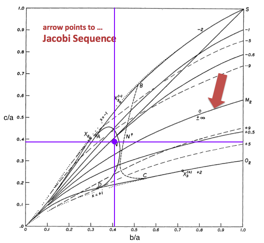
The subscript "EFE" on Ω and λ means that the relevant frequency is given in units that have been adopted in [EFE], that is, in units of <math>~[\pi G\rho]^{1 / 2}</math>. In Figure 1a, the solid purple circular marker (where the pair of purple lines cross) identifies the location of this model in the "c/a versus b/a" diagram that appears as Figure 2 on p. 902 of S. Chandrasekhar (1965); essentially the same diagram appears in §49 (p. 147) of [EFE].
See Also
- Discussion of Ou's Riemann-Like Ellipsoids

|
|---|
|
© 2014 - 2021 by Joel E. Tohline |

