User:Tohline/Appendix/Ramblings/FourierSeries

Fourier Series

Representations

The following Fourier series representations have been drawn primarily from pp. 458 - 460 of the 1971 (19^th) edition of the CRC's Standard Mathematical Tables, published by the Chemical Rubber Co., Cleveland, Ohio, U.S.A.

Standard

If <math>~f(x)</math> is a bounded periodic function of period <math>~2L</math>, it may be represented by the Fourier series,

Standard Fourier Series Expression
<math>~f(x)</math> <math>~=</math> <math>~ \frac{a_0}{2} + \sum_{n=1}^{\infty} \biggl[ a_n\cos \biggl(\frac{n\pi x}{L}\biggr) + b_n\sin \biggl(\frac{n\pi x}{L}\biggr) \biggr] \, , </math>

where,

<math>~a_n</math>	<math>~=</math>	<math>~ \frac{1}{L} \int_{-L}^{L} f(x) \cos\biggl( \frac{n\pi x}{L} \biggr) dx </math>		for	<math>~n = 0, 1, 2, 3, \dots \, ;</math>
<math>~b_n</math>	<math>~=</math>	<math>~ \frac{1}{L} \int_{-L}^{L} f(x) \sin\biggl( \frac{n\pi x}{L} \biggr) dx </math>		for	<math>~n = 1, 2, 3, \dots </math>

LaTeX mathematical expressions cut-and-pasted directly from NIST's Digital Library of Mathematical Functions

As an additional primary point of reference, note that according to §1.8(i) of NIST's Digital Library of Mathematical Functions, a Fourier Series is defined as follows: <math>~f(x)</math> <math>~=</math> <math>~\tfrac{1}{2}a_{0}+\sum^{\infty}_{n=1}\biggl[ a_{n}\cos\bigl(nx\bigr)+b_{n}\sin\bigl(nx\bigr) \biggr],</math> <math>~a_n</math> <math>~=</math> <math>~\frac{1}{\pi}\int^{\pi}_{-\pi}f(x)\cos\bigl(nx\bigr)\mathrm{d}x,</math> <math>~b_n</math> <math>~=</math> <math>~\frac{1}{\pi}\int^{\pi}_{-\pi}f(x)\sin\bigl(nx\bigr)\mathrm{d}x.</math>

Alternate

Alternatively, if we set <math>~a_n = c_n \cos\phi_n</math> and <math>~b_n = - c_n \sin\phi_n</math>, then,

<math>~a_n\cos \biggl(\frac{n\pi x}{L}\biggr) + b_n\sin \biggl(\frac{n\pi x}{L}\biggr) </math>	<math>~=</math>	<math>~ c_n \cos\phi_n \cos \biggl(\frac{n\pi x}{L}\biggr) - c_n \sin\phi_n \sin \biggl(\frac{n\pi x}{L}\biggr) </math>
	<math>~=</math>	<math>~ c_n \cos \biggl(\frac{n\pi x}{L} + \phi_n \biggr) \, , </math>

in which case we may rewrite the Fourier series expression in the form,

Alternate Fourier Series Expression
<math>~f(x)</math> <math>~=</math> <math>~ \frac{a_0}{2} + \sum_{n=1}^{\infty} c_n\cos \biggl(\frac{n\pi x}{L} + \phi_n\biggr) \, , </math>

where,

<math>~c_n = \sqrt{a_n^2 + b_n^2}</math>

and

<math>~\phi_n = \tan^{-1}\biggl(\frac{-b_n}{a_n}\biggr) \, .</math>

Complex

Here we make use of the exponential/complex relation — also referred to as Euler's equation,

<math>~e^{i\alpha} = \cos\alpha + i \sin\alpha \, ,</math>     <math>~\Rightarrow</math>     <math>~e^{-i\alpha} = \cos\alpha - i \sin\alpha \, ,</math>

in which case we may write,

<math>~\cos\alpha = \frac{1}{2} \biggl[ e^{i\alpha} + e^{-i\alpha}\biggr] \, ,</math>

and

<math>~\sin\alpha = \frac{1}{2i} \biggl[ e^{i\alpha} - e^{-i\alpha}\biggr]\, .</math>

Employing these definitions of the trigonometric relations <math>~\cos\alpha</math> and <math>~\sin\alpha</math>, the standard representation of the Fourier series may be rewritten as,

Complex Fourier Series Expression
<math>~f(x)</math> <math>~=</math> <math>~ \frac{1}{2}\sum_{n = -\infty}^{n = + \infty} d_n e^{i\omega_n x} \, , </math>

where, for <math>~n = 0, \pm 1, \pm 2, \pm 3, \dots~</math>,

<math>~\omega_n</math>

<math>~=</math>

<math>~ \frac{n\pi }{L} \, , </math>

and the complex coefficients,

<math>~d_n = a_{n} -i b_{n} </math>	<math>~=</math>	<math>~ \frac{1}{L} \int_{-L}^{L} f(x) \cos\biggl( \frac{n\pi x}{L} \biggr) dx - i\frac{1}{L} \int_{-L}^{L} f(x) \sin\biggl( \frac{n\pi x}{L} \biggr) dx </math>
	<math>~=</math>	<math>~ \frac{1}{L} \int_{-L}^{L} f(x) \biggl[ \cos\biggl( \frac{n\pi x}{L} \biggr) - i\sin\biggl( \frac{n\pi x}{L} \biggr)\biggr] dx </math>
	<math>~=</math>	<math>~ \frac{1}{L} \int_{-L}^{L} f(x)e^{-i\omega_n x} dx \, . </math>

Let's demonstrate that this rewritten (complex) expression for <math>~f(x)</math> matches the standard Fourier series expression. First, we will refer to the above standard definitions of <math>~a_n</math> and <math>~b_n</math> as, respectively, <math>~a_{|n|}</math> and <math>~b_{|n|}</math>, and recognize that, as the summation is extended to negative numbers, the following mapping is appropriate:

<math>~a_n ~ \rightarrow ~ a_{|n|}</math>	and	<math>~b_n ~ \rightarrow ~ b_{|n|} \, ,</math>	for	<math>~n > 0 \, ;</math>
<math>~a_n ~ \rightarrow ~ a_{|n|}</math>	and	<math>~b_n ~ \rightarrow ~ - b_{|n|} \, ,</math>	for	<math>~n < 0 \, .</math>

Hence, we have,

<math>~2f(x)</math>	<math>~=</math>	<math>~ \sum_{n = -\infty}^{n = + \infty} (a_n - ib_n)e^{i\omega_n x} </math>
	<math>~=</math>	<math>~ \sum_{n = 1}^{n = + \infty} (a_{|n|} - ib_{|n|})e^{i\omega_{|n|} x} + a_0 + \sum_{n = \infty}^{n = 1} (a_{|n|} + ib_{|n|})e^{- i\omega_{|n|} x} </math>
	<math>~=</math>	<math>~ \sum_{n = 1}^{n = + \infty} (a_{|n|} - ib_{|n|}) [ \cos (\omega_{|n|} x) + i\sin (\omega_{|n|} x)] + a_0 + \sum_{n = 1}^{n = \infty} (a_{|n|} + ib_{|n|}) [ \cos (\omega_{|n|} x) - i\sin (\omega_{|n|} x)] </math>
	<math>~=</math>	<math>~ a_0 + \sum_{n = 1}^{n = + \infty}\biggl\{ (a_{|n|} - ib_{|n|}) [ \cos (\omega_{|n|} x) + i\sin (\omega_{|n|} x)] + (a_{|n|} + ib_{|n|}) [ \cos (\omega_{|n|} x) - i\sin (\omega_{|n|} x)] \biggr\} </math>
	<math>~=</math>	<math>~ a_0 + \sum_{n = 1}^{n = + \infty}\biggl\{2a_{|n|} \cos (\omega_{|n|} x) + 2b_{|n|} \sin (\omega_{|n|} x)] \biggr\} </math>
<math>~\Rightarrow ~~~ f(x)</math>	<math>~=</math>	<math>~ \frac{a_0}{2} + \sum_{n = 1}^{n = + \infty}\biggl\{a_{|n|} \cos (\omega_{|n|} x) + b_{|n|} \sin (\omega_{|n|} x)] \biggr\} \, . </math>

Q.E.D.

From Williams & Tohline (1987)

This discussion parallels the discussion of a Fourier series analysis that was presented by H. A. Williams & J. E. Tohline (1987, ApJ, 315, 594) — see especially their §III — in the context of their discussion of nonlinear dynamic instabilities in rotating polytropes.

Standard Setup

A useful way of analyzing the growth and pattern speed of nonaxisymmetric structures is to Fourier transform the (discrete) density distribution, <math>~\rho(\theta_L)</math>, in angle space, <math>~\theta_L = L \delta\theta</math>, where, <math>~\delta\theta \equiv 2\pi/L_\mathrm{max}</math>. On the discrete angular grid, the Fourier transform equations are

<math>~a_m</math>	<math>~=</math>	<math>~ \frac{2}{L_\mathrm{max}} \cdot \sum_{L=1}^{L_\mathrm{max}} \rho(\theta_L) \cos(m\theta_L) \, , </math>
<math>~b_m</math>	<math>~=</math>	<math>~ \frac{2}{L_\mathrm{max}} \cdot \sum_{L=1}^{L_\mathrm{max}} \rho(\theta_L) \sin(m\theta_L) \, . </math>

Notice that, <math>~a_0 = 2\bar\rho</math>, where <math>~\bar\rho</math> is the average density. The density function can be reconstructed via the expression,

<math>~\rho(\theta_L)</math>

<math>~=</math>

<math>~ \frac{a_0}{2} + \sum_{m=1}^{L_\mathrm{max}/2} \biggl[ a_m \cos(m\theta_L) + b_m\sin(m\theta_L) \biggr] \, , </math>

so the <math>~a_m</math> and <math>~b_m</math> coefficients can, and should be, interpreted as amplitudes of various Fourier modes <math>~(m)</math>.

Example #1

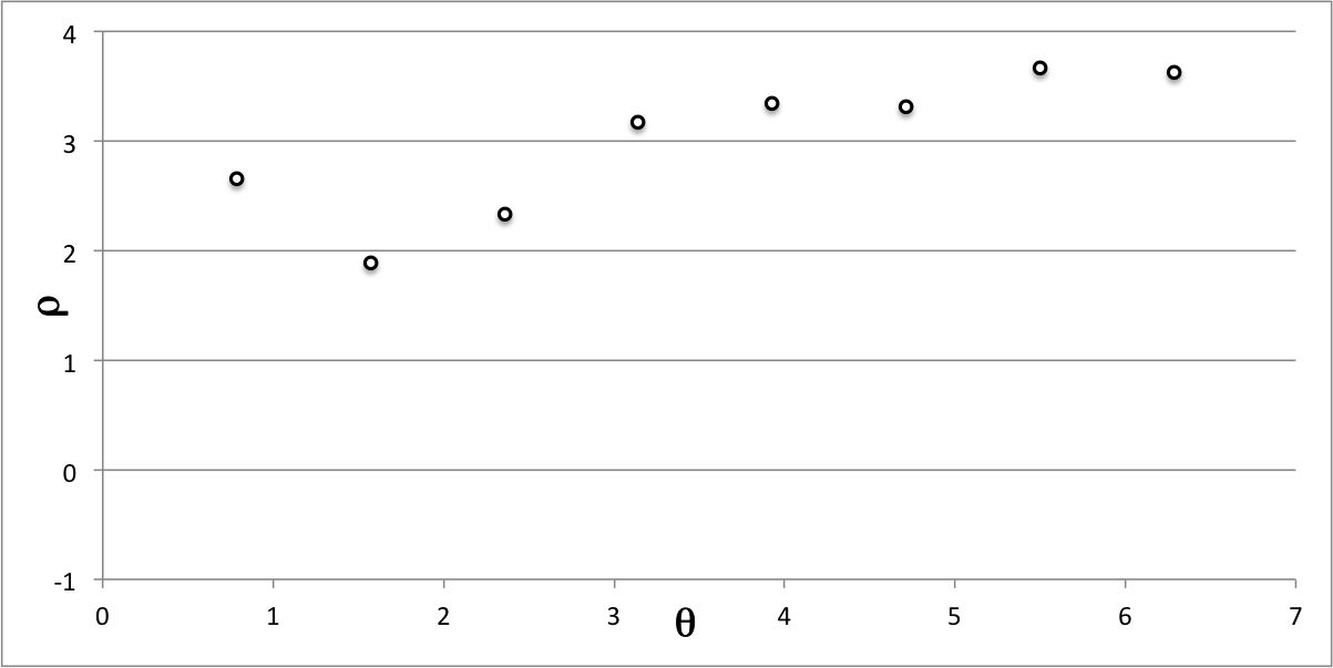
Here we are interested in examining a density distribution, <math>~\rho(\theta)</math>, that varies smoothly over the angular coordinate interval, <math>~0 < \theta \le 2\pi</math>, and whose distribution is strictly periodic over all other <math>~2\pi</math> intervals. Suppose that we do not have a functional specification of this continuous density distribution but, instead, are given the value of the density, <math>~\rho_i(\theta_L)</math>, at <math>~L_\mathrm{max} = 8</math>, equally spaced discrete angular-coordinate locations, <math>~\theta_L = (2\pi L/L_\mathrm{max})</math>.

Figure 1a

Specifically, suppose that the eight values of the the density and corresponding discrete angular-coordinate locations are those identified by the eight open circular markers in Figure 1a and listed, respectively, in columns 3 and 2 of Table 1. Feeding these eight discrete values of <math>~\rho_i</math> and <math>~\theta_L</math> into the above Fourier transform equations, we have determined the <math>~a_m</math> and <math>~b_m</math> coefficient values and have listed them in columns 5 and 6, respectively, of Table 1.

Table 1:  Data Associated with Example #1
Discrete Evaluation				Fourier Amplitudes				Reconstruction
<math>~L</math>	<math>~\theta_L = \frac{2\pi L}{L_\mathrm{max}}</math>	<math>~\rho_i(\theta_L)</math>		<math>~m</math>	<math>~a_m</math>	<math>~b_m</math>		<math>~\rho(\theta_L)</math>
				<math>~0</math>	6.0000	0.0000		<math>~</math>
<math>~1</math>	<math>~0.7854</math>	<math>~2.6595</math>		<math>~1</math>	0.2318	-0.7133		<math>~2.6595</math>
<math>~2</math>	<math>~1.5708</math>	<math>~1.8867</math>		<math>~2</math>	0.4000	0.0000		<math>~1.8867</math>
<math>~3</math>	<math>~2.3562</math>	<math>~2.3317</math>		<math>~3</math>	0.0000	0.0000		<math>~2.3317</math>
<math>~4</math>	<math>~3.1416</math>	<math>~3.1682</math>		<math>~4</math>	0.0000	0.0000		<math>~3.1682</math>
<math>~5</math>	<math>~3.9270</math>	<math>~3.3405</math>		<math>~5</math>	0.0000	0.0000		<math>~3.3405</math>
<math>~6</math>	<math>~4.7124</math>	<math>~3.3133</math>		<math>~6</math>	0.4000	0.0000		<math>~3.3133</math>
<math>~7</math>	<math>~5.4978</math>	<math>~3.6683</math>		<math>~7</math>	0.2318	+0.7133		<math>~3.6683</math>
<math>~8</math>	<math>~6.2832</math>	<math>~3.6318</math>		<math>~8</math>	6.0000	0.0000		<math>~3.6318</math>

Notice the following:

• Given that the initial discrete density distribution, <math>~\rho_i(\theta_L)</math>, is real (as opposed to complex) and has been given only at <math>~L_\mathrm{max} = 8</math> angular locations over the coordinate range, <math>~0 < \theta_L \le 2\pi</math> — it repeats in a periodic fashion outside of this range — the Fourier series can have, at most, <math>~L_\mathrm{max} = 8</math> independent coefficient values. In Table 1, the cells with light-blue backgrounds contain these eight independent values. Elaboration: For each Fourier mode over the range, <math>~1 \le m \le (\tfrac{1}{2}L_\mathrm{max} - 1)</math>, there are two relevant, independent coefficients, namely, <math>~a_m</math> and <math>~b_m</math>, giving, in our Example #1, six of the expected eight coefficient values. The other two unique coefficient values arise from <math>~m = 0</math> and <math>~m = \tfrac{1}{2}L_\mathrm{max}</math>. In both of these "edge" cases, only the <math>~a_m</math> coefficient provides relevant information; <math>~b_m</math> is irrelevant because, when <math>~m=0</math>, the argument of the sine function is always zero, and when <math>~m = \tfrac{1}{2}L_\mathrm{max}</math>, the argument of the sine function is <math>~m\theta_L = \tfrac{1}{2}L_\mathrm{max} \cdot 2\pi L/L_\mathrm{max} = \pi L</math>.

According to the standard setup presented above, for this particular example analysis the density reconstruction is obtained via the expression,

<math>~\rho(\theta_L)</math>	<math>~=</math>	<math>~\frac{a_0}{2} + a_1\cos(\theta_L) + b_1\sin(\theta_L) + a_2\cos(2\theta_L) + b_2\sin(2\theta_L) + a_3\cos(3\theta_L) + b_3\sin(3\theta_L) + a_4\cos(4\theta_L) </math>
	<math>~=</math>	<math>~ 3 + [0.2318\cos(\theta_L) - 0.7133\sin(\theta_L)] + 0.4\cos(2\theta_L) \, . </math>

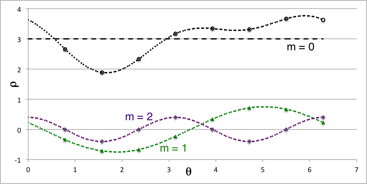
The values of <math>~\rho(\theta_L)</math> listed in the last column (column 7) of Table 1 have been calculated from this expression and, indeed, across the board they match the originally specified, discrete values of <math>~\rho_i(\theta_L)</math>. Notice, however, that this last expression not only can be used to generate correct values of the density at the originally identified discrete angular coordinate locations, it also offers an analytic prescription of a continuous function for the density distribution across the entire angular-coordinate domain. In addition to redisplaying the initially specified discrete values of the density (open circular markers) from Figure 1a, Figure1b presents this continuous function's modal decomposition. Specifically, the horizontal (black) dashed line is the <math>~m = 0</math> contribution; the green curve shows the sum of the two (sine and cosine) terms that represent the <math>~m=1</math> component; and the purple curve displays the <math>~m = 2</math> contribution.

Figure 1b

When added together, these three modal contributions give the continuous density distribution depicted by the dotted black curve in Figure 1b; as desired, this continuous curve runs through all eight initially specified discrete values of the density.

Alternatively, Introduce Phase Shift

Alternatively, we can switch from the Fourier series coefficients, <math>~a_m</math> and <math>~b_m</math>, to the coefficient/phase definitions, <math>~c_m</math> and <math>~\phi_m</math>, such that,

<math>~c_m</math>

<math>~=</math>

<math>~ [a_m^2 + b_m^2]^{1 / 2} \, , </math>

and,

<math>~\phi_m</math>	<math>~=</math>	<math>~ \tan^{-1}\biggl( \frac{-b_m}{a_m} \biggr) \, , </math>	for …	<math>~a_m > 0 \, ,</math>
<math>~\phi_m</math>	<math>~=</math>	<math>~ \tan^{-1}\biggl( \frac{-b_m}{a_m} \biggr) +\pi \, , </math>	for …	<math>~a_m < 0 \, .</math>

Notice that, when <math>~a_m = 0</math>, <math>~\tan^{-1}(-b_m/a_m) = \pi/2</math>. Using <math>~c_m</math> and <math>~\phi_m</math>, the discrete density distribution can be exactly reconstructed via the Fourier series,

<math>~\rho(\theta_L)</math>

<math>~=</math>

<math>~ \frac{c_0}{2} + \sum_{m=1}^{L_\mathrm{max}/2} c_m \cos\biggl[m\theta_L + \phi_m\biggr] \, . </math>

In Table 2, we have reprinted the values of the coefficients, <math>~a_m</math> and <math>~b_m</math>, that were calculated above in connection with "Example #1", and, from this data for each Fourier mode, we have calculated/tabulated the corresponding values of <math>~c_m</math> and <math>~\phi_m</math>. It is straightforward to demonstrate that the eight discrete values of the density, <math>~\rho_(\theta_L)</math>, that are reconstructed from these new coefficient/phase values precisely match the eight density values, <math>~\rho_i(\theta_L)</math>, that served as input to our "Example #1" discussion.

Table 2
<math>~m</math>	<math>~a_m</math>	<math>~b_m</math>	<math>~c_m</math>	<math>~\phi_m</math>
<math>~0</math>	<math>~6</math>	<math>~0</math>	<math>~6</math>	<math>~0</math>
<math>~1</math>	<math>~0.2318</math>	<math>~-0.7133</math>	<math>~0.7500</math>	<math>~0.4\pi</math>
<math>~2</math>	<math>~0.4</math>	<math>~0.0</math>	<math>~0.4</math>	<math>~0.0</math>
<math>~3</math>	<math>~0.0</math>	<math>~0.0</math>	<math>~0.0</math>	undefined
<math>~4</math>	<math>~0.0</math>	<math>~0.0</math>	<math>~0.0</math>	undefined

Example #2

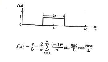
The figure/equation pair displayed here, on the right, is an example of a "Fourier expansion for a basic periodic function" that has been presented on p. 464 of the CRC Standard Mathematical Tables (19th Edition). The following derivation, analysis, and discussion has been motivated by this published CRC example.

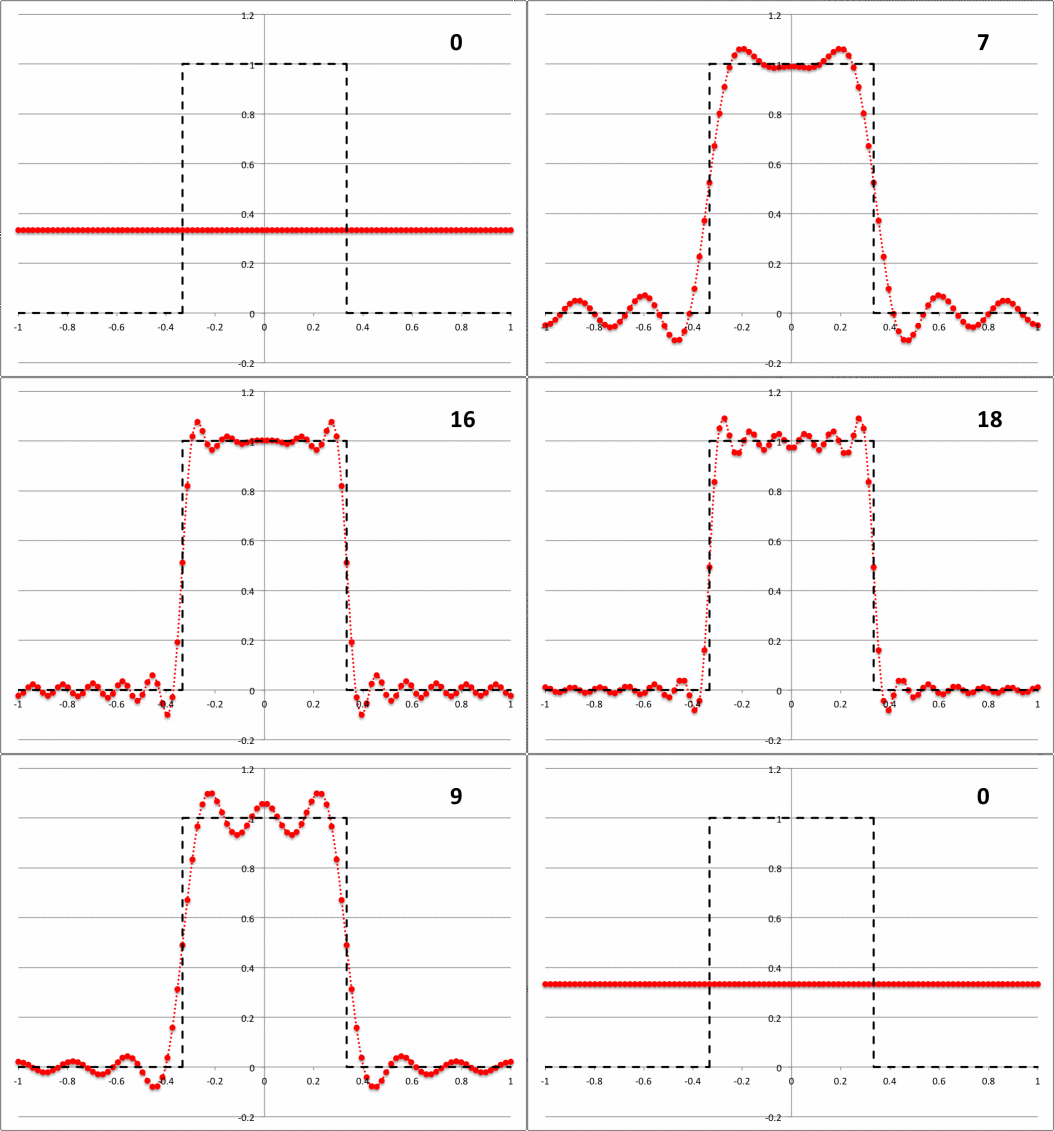
Referring back to the standard representation presented above, suppose that <math>~f(x)</math> is a square wave (unity amplitude) that extends over the range <math>~\pm c</math>, where, <math>~c < L</math>. (The dashed-black curve in Figure 2, below, displays one cycle of this function for the specific case of c/L = 1/3.) Replacing <math>~x</math> by the angle,

<math>~\theta \equiv \frac{n\pi x}{L} \, ,</math>

the two coefficients are (for all n > 0),

<math>~a_n</math>	<math>~=</math>	<math>~ \frac{1}{L} \int_{-c}^{c} \cos\biggl( \frac{n\pi x}{L} \biggr) dx </math>
	<math>~=</math>	<math>~ \biggl( \frac{1}{n\pi} \biggr) \int_{-(n\pi c/L)}^{(n\pi c/L)} \cos ( \theta ) d\theta </math>
	<math>~=</math>	<math>~ \biggl( \frac{1}{n\pi} \biggr) \biggl[\sin ( \theta ) \biggr]_{-(n\pi c/L)}^{(n\pi c/L)} </math>
	<math>~=</math>	<math>~ \biggl( \frac{2}{n\pi} \biggr) \sin \biggl( \frac{n\pi c}{L} \biggr) \, , </math>
<math>~b_n</math>	<math>~=</math>	<math>~ \frac{1}{L} \int_{-c}^{c} \sin\biggl( \frac{n\pi x}{L} \biggr) dx </math>
	<math>~=</math>	<math>~ \biggl( \frac{1}{n\pi} \biggr) \int_{-(n\pi c/L)}^{(n\pi c/L)} \sin ( \theta ) d\theta </math>
	<math>~=</math>	<math>~ -\biggl( \frac{1}{n\pi} \biggr) \biggl[\cos ( \theta ) \biggr]_{-(n\pi c/L)}^{(n\pi c/L)} </math>
	<math>~=</math>	<math>~ 0 \, . </math>

For the special case of <math>~n = 0</math>, we have,

<math>~a_0 = \frac{1}{L}\int_{-c}^c dx = \frac{2c}{L} \, ,</math>

and

<math>~b_0 = 0 \, .</math>

Hence, the Fourier series expression for the square-wave function, itself, is,

<math>~f(x)</math>	<math>~=</math>	<math>~ \frac{a_0}{2} + \sum_{n=1}^{\infty} \biggl[ a_n\cos \biggl(\frac{n\pi x}{L}\biggr) + b_n\sin \biggl(\frac{n\pi x}{L}\biggr) \biggr] </math>
	<math>~=</math>	<math>~ \frac{c}{L} + \sum_{n=1}^{\infty} \biggl( \frac{2}{n\pi} \biggr) \sin \biggl( \frac{n\pi c}{L} \biggr) \cos \biggl(\frac{n\pi x}{L}\biggr) \, . </math>

Figure 2:   Approximate Series Expressions for a Square-Wave <math>~\frac{c}{L} = \frac{1}{3}</math>
The dotted-red curve displays the behavior of the (approximate) function <math>~f(x)</math>, as the series expression is truncated for various values of the index, <math>~n</math>, as indicated by the (time-varying) integer legend. The dashed-black "square wave" shows the input function, which should be the behavior of <math>~f(x)</math> when the series expression includes an infinite number of terms.

Notice the following:

1. If we define,

   <math>~\alpha_n \equiv \frac{n\pi c}{L} \, ,</math>

   then, as a function of <math>~\alpha</math>, the Fourier mode amplitude is,

   <math>~a_n(\alpha_n)</math>

   <math>~=</math>

   <math>~\biggl( \frac{2c}{L} \biggr) \frac{\sin \alpha_n}{\alpha_n} = \biggl( \frac{2c}{L} \biggr) \mathrm{sinc}(\alpha_n) \, .</math>

2. The inverse transform may also then be rewritten as,

   <math>~f(x)</math>

   <math>~=</math>

   <math>~ \frac{2c}{L}\biggl[ \frac{1}{2} +\sum_{n=1}^{\infty} \mathrm{sinc}(\alpha_n) \cos \biggl(\frac{n\pi x}{L}\biggr) \biggr] \, . </math>

3. The sinc function goes to zero each time its argument, <math>~\alpha_n</math>, is an integer multiple of π. This means that the first zero arises at <math>~n = L/c</math>, if <math>~L</math> is an integer-multiple of <math>~c</math>. This also means that the discrete array that marks the Fourier mode amplitude, <math>~a_n</math>, will resolve the central amplitude peak only if <math>~c/L \ll 1</math>.

Example #3

Now, let's reverse the example provided as Example #2. Specifically, let's look for the Fourier series expression for the function,

<math>~g(x) \equiv c~\mathrm{sinc}(\alpha) \, ,</math>

for <math>~\alpha \equiv \pi x/c</math>, over the range, <math>~-m \pi \le \alpha_n \le + m \pi</math>. Furthermore, we will assume that <math>~g(x)</math> is a periodic function of period <math>~2mc</math>, in which case it may be represented by the Fourier series,

<math>~g(x)</math>

<math>~=</math>

<math>~ \frac{a_0}{2} + \sum_{n=1}^{\infty} \biggl[ a_n\cos \biggl(\frac{n\pi x}{L}\biggr) + b_n\sin \biggl(\frac{n\pi x}{L}\biggr) \biggr] \, , </math>

where,

<math>~a_n</math>	<math>~=</math>	<math>~ \frac{1}{L} \int_{-L}^{L} g(x) \cos\biggl( \frac{n\pi x}{L} \biggr) dx </math>		for	<math>~n = 0, 1, 2, 3, \dots \, ;</math>
<math>~b_n</math>	<math>~=</math>	<math>~ \frac{1}{L} \int_{-L}^{L} g(x) \sin\biggl( \frac{n\pi x}{L} \biggr) dx </math>		for	<math>~n = 1, 2, 3, \dots </math>

One-Dimensional Aperture

General Concept

Hence, we have,

<math>~A(y_1)</math>	<math>~=</math>	<math>~A_0 \sum_j a_j e^{-i[2\pi y_1 Y_j/(\lambda L)]} \, , </math>
	<math>~=</math>	<math>~A_0 \sum_j a_j \biggl[ \cos\biggl(\frac{2\pi y_1 Y_j}{\lambda L} \biggr) - i \sin\biggl(\frac{2\pi y_1 Y_j}{\lambda L} \biggr) \biggr] \, , </math>

where, now, <math>~A_0 = e^{i2\pi L/\lambda}</math>. When written in this form, it should immediately be apparent why discrete Fourier transform techniques (specifically FFT techniques) are useful tools for evaluation of the complex amplitude, <math>~A</math>.

See Also

• Tohline, J. E., (2008) Computing in Science & Engineering, vol. 10, no. 4, pp. 84-85 — Where is My Digital Holographic Display? [ PDF ]

© 2014 - 2021 by Joel E. Tohline |   H_Book Home   |   YouTube   | Appendices: | Equations | Variables | References | Ramblings | Images | myphys.lsu | ADS | Recommended citation:   Tohline, Joel E. (2021), The Structure, Stability, & Dynamics of Self-Gravitating Fluids, a (MediaWiki-based) Vistrails.org publication, https://www.vistrails.org/index.php/User:Tohline/citation