Difference between revisions of "User:Tohline/Appendix/Ramblings/Azimuthal Distortions"
(→Analyzing Azimuthal Distortions: Finished explaining four panels of our Figure 1) |
|||
| Line 4: | Line 4: | ||
{{LSU_HBook_header}} | {{LSU_HBook_header}} | ||
In what follows, we will draw heavily from two publications: [http://adsabs.harvard.edu/abs/1990ApJ...361..394T J. E. Tohline & I. Hachisu (1988, ApJ, 361, 394)] — hereafter, TH88 — and [http://adsabs.harvard.edu/abs/2011Ap%26SS.334....1H K. Hadley & J. N. Imamura (2011a, ''Astrophysics and Space Science'', 334, 1)] — hereafter, HI11a. | |||
==Adopted Notation== | ==Adopted Notation== | ||
Beginning with equation (2) of [http://adsabs.harvard.edu/abs/1990ApJ...361..394T TH88] but ignoring variations in the vertical coordinate direction, the mass density is given by the expression, | |||
<div align="center"> | <div align="center"> | ||
<table border="0" cellpadding="5" align="center"> | <table border="0" cellpadding="5" align="center"> | ||
| Line 143: | Line 144: | ||
<tr> | <tr> | ||
<td align="right"> | <td align="right"> | ||
<math>~\biggl[ \frac{\rho}{\rho_0} | <math>~\biggl[ \frac{\delta\rho}{\rho_0}\biggr]_\mathrm{rot} \equiv \biggl[ \frac{\rho}{\rho_0} - 1 \biggr]e^{im\Omega_p t}</math> | ||
</td> | </td> | ||
<td align="center"> | <td align="center"> | ||
| Line 156: | Line 157: | ||
whose relative amplitude — with a radial structure as specified inside the curly braces — is undergoing a uniform exponential growth but is otherwise unchanging. | whose relative amplitude — with a radial structure as specified inside the curly braces — is undergoing a uniform exponential growth but is otherwise unchanging. | ||
Figure 1 illustrates how the behavior of each factor in this expression can reveal itself during a numerical simulation that follows the time-evolutionary development of an unstable, nonaxisymmetric eigenmode. The initial model for this depicted evolution | Drawing from figure 2 of [http://adsabs.harvard.edu/abs/1990ApJ...361..394T TH88], our Figure 1, immediately below, illustrates how the behavior of each factor in this expression can reveal itself during a numerical simulation that follows the time-evolutionary development of an unstable, nonaxisymmetric eigenmode. The initial model for this depicted evolution (model O3 from Table 1 of [http://adsabs.harvard.edu/abs/1990ApJ...361..394T TH88]) is a zero-mass — that is, it is a [[User:Tohline/Apps/PapaloizouPringleTori#Massless_Polytropic_Tori|Papaloizou-Pringle like torus]] — with [[User:Tohline/SR#Barotropic_Structure|polytropic index]],<math>~n = 3</math>, and a rotation-law profile defined by [[User:Tohline/AxisymmetricConfigurations/SolutionStrategies#Simple_Rotation_Profile_and_Centrifugal_Potential|uniform specific angular momentum]]. | ||
* The top-left panel shows how, at any radial location, the phase angle, <math>~\phi_1/(2\pi)</math>, for the <math>~m=1</math> eigenmode, varies with time, <math>~t/t_\mathrm{rot}</math>, where, <math>~t_\mathrm{rot} \equiv 2\pi/\Omega_0</math> is the rotation period at the density maximum; | |||
<math>~t_\mathrm{rot} \equiv | * Using a semi-log plot, the top-right panel shows the exponential growth of the amplitude of three separate modes: The dominant unstable mode, displaying the largest amplitude, is <math>~m = 1</math>. | ||
</ | * Using a semi-log plot (log amplitude versus fractional radius, <math>~\varpi/r_+</math>), the bottom-left panel displays the shape of the eigenfunction, <math>~f_1(\varpi)</math>, for the unstable, <math>~m=1</math> mode; | ||
* The bottom-right panel displays the radial dependence of the equatorial-plane phase angle, <math>~\phi_1(\varpi)</math>, for the unstable, <math>~m=1</math> mode; this is what [http://adsabs.harvard.edu/abs/2011Ap%26SS.334....1H TI11a] refer to as the "constant phase loci." | |||
Revision as of 23:05, 5 January 2016
Analyzing Azimuthal Distortions

|
|---|
| | Tiled Menu | Tables of Content | Banner Video | Tohline Home Page | |
In what follows, we will draw heavily from two publications: J. E. Tohline & I. Hachisu (1988, ApJ, 361, 394) — hereafter, TH88 — and K. Hadley & J. N. Imamura (2011a, Astrophysics and Space Science, 334, 1) — hereafter, HI11a.
Adopted Notation
Beginning with equation (2) of TH88 but ignoring variations in the vertical coordinate direction, the mass density is given by the expression,
|
<math>~\rho</math> |
<math>~=</math> |
<math>~\rho_0 \biggl[ 1 + f(\varpi)e^{-i(\omega t - m\phi)} \biggr] \, ,</math> |
where it is understood that <math>~\rho_0</math>, which defines the structure of the initial axisymmetric equilibrium configuration, is generally a function of the cylindrical radial coordinate, <math>~\varpi</math>.
Using the subscript, <math>~m</math>, to identify the time-invariant coefficients and functions that characterize the intrinsic eigenvector of each azimuthal eigen-mode, and acknowledging that the associated eigenfrequency will in general be imaginary, that is,
|
<math>~\omega_m</math> |
<math>~=</math> |
<math>~\omega_R + i\omega_I \, ,</math> |
we expect each unstable mode to display the following behavior:
|
<math>~\biggl[ \frac{\rho}{\rho_0} - 1 \biggr]</math> |
<math>~=</math> |
<math>~f_m(\varpi)e^{-i[\omega_R t + i \omega_I t - m\phi_m(\varpi)]} </math> |
|
|
<math>~=</math> |
<math>~\biggl\{ f_m(\varpi)e^{-im\phi_m(\varpi)}\biggr\} e^{-i\omega_R t } \cdot e^{\omega_I t} </math> |
|
|
<math>~=</math> |
<math>~\biggl\{ f_m(\varpi)e^{-i[\omega_R t + m\phi_m(\varpi)]} \biggr\} e^{\omega_I t} \, .</math> |
Adopting Kojima's (1986) notation, that is, defining,
|
<math>~y_1 \equiv \frac{\omega_R}{\Omega_0} - m</math> |
and |
<math>~y_2 \equiv \frac{\omega_I}{\Omega_0} \, ,</math> |
the eigenvector's behavior can furthermore be described by the expression,
|
<math>~\biggl[ \frac{\rho}{\rho_0} - 1 \biggr]</math> |
<math>~=</math> |
<math>~\biggl\{ f_m(\varpi)e^{-i[(y_1+m) (\Omega_0 t) + m\phi_m(\varpi)]} \biggr\} e^{y_2 (\Omega_0 t)} </math> |
|
|
<math>~=</math> |
<math>~\biggl\{ f_m(\varpi)e^{-im[(y_1/m+1) (\Omega_0 t) + \phi_m(\varpi)]} \biggr\} e^{y_2 (\Omega_0 t)} \, .</math> |
Note that, as viewed from a frame of reference that is rotating with the mode pattern frequency,
<math>\Omega_p \equiv \frac{\omega_R}{m} = \Omega_0\biggl(\frac{y_1}{m}+1\biggr) \, ,</math>
we should find an eigenvector of the form,
|
<math>~\biggl[ \frac{\delta\rho}{\rho_0}\biggr]_\mathrm{rot} \equiv \biggl[ \frac{\rho}{\rho_0} - 1 \biggr]e^{im\Omega_p t}</math> |
<math>~=</math> |
<math>~\biggl\{ f_m(\varpi)e^{-im[\phi_m(\varpi)]} \biggr\} e^{y_2 (\Omega_0 t)} \, ,</math> |
whose relative amplitude — with a radial structure as specified inside the curly braces — is undergoing a uniform exponential growth but is otherwise unchanging.
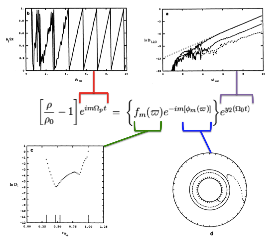
Drawing from figure 2 of TH88, our Figure 1, immediately below, illustrates how the behavior of each factor in this expression can reveal itself during a numerical simulation that follows the time-evolutionary development of an unstable, nonaxisymmetric eigenmode. The initial model for this depicted evolution (model O3 from Table 1 of TH88) is a zero-mass — that is, it is a Papaloizou-Pringle like torus — with polytropic index,<math>~n = 3</math>, and a rotation-law profile defined by uniform specific angular momentum.
- The top-left panel shows how, at any radial location, the phase angle, <math>~\phi_1/(2\pi)</math>, for the <math>~m=1</math> eigenmode, varies with time, <math>~t/t_\mathrm{rot}</math>, where, <math>~t_\mathrm{rot} \equiv 2\pi/\Omega_0</math> is the rotation period at the density maximum;
- Using a semi-log plot, the top-right panel shows the exponential growth of the amplitude of three separate modes: The dominant unstable mode, displaying the largest amplitude, is <math>~m = 1</math>.
- Using a semi-log plot (log amplitude versus fractional radius, <math>~\varpi/r_+</math>), the bottom-left panel displays the shape of the eigenfunction, <math>~f_1(\varpi)</math>, for the unstable, <math>~m=1</math> mode;
- The bottom-right panel displays the radial dependence of the equatorial-plane phase angle, <math>~\phi_1(\varpi)</math>, for the unstable, <math>~m=1</math> mode; this is what TI11a refer to as the "constant phase loci."
|
Figure 1 |
|
Four panels extracted† from figure 2, p. 252 of J. W. Woodward, J. E. Tohline & I. Hachisu (1994)
"The Stability of Thick, Self-gravitating Disks in Protostellar Systems"
ApJ, vol. 420, pp. 247-267 © American Astronomical Society |
| †As displayed here, the layout of figure panels (a, b, c, d) has been modified from the original publication layout; otherwise, each panel is unmodified. |
Empirical Construction of Eigenvector
|
Figure 2 |
|
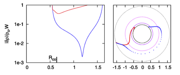
Panel pair extracted† without modification from the top-most segment of Figure 13, p. 12 of K. Hadley & J. N. Imamura (2011a)
"Nonaxisymmetric Instabilities of Self-Gravitating Disks. I Toroids"
Astrophysics and Space Science, 334, 1 - 26 © Springer Science+Business Media B.V. |
| †This pair of plots also appears, by itself, as Figure 6 on p. 12 of K. Hadley & J. N. Imamura (2011a). |
First, specify a "midway" radial location, <math>~r_- < r_\mathrm{mid} < r_+ \, ,</math> at which the density fluctuation is smallest. Then define a function of the form,
|
<math>~f(\varpi)</math> |
<math>~=</math> |
<math>~\tanh^{-1}\biggl[1 - 2 \biggl( \frac{\varpi - r_-}{r_\mathrm{mid}-r_-} \biggr) \biggr]</math> |
for |
<math>r_- < \varpi < r_\mathrm{mid} \, ;</math> |
| and | ||||
|
<math>~f(\varpi)</math> |
<math>~=</math> |
<math>~\tanh^{-1}\biggl[1 - 2 \biggl( \frac{\varpi - r_+}{r_\mathrm{mid}-r_+} \biggr) \biggr]</math> |
for |
<math>r_\mathrm{mid} < \varpi < r_+ \, .</math> |
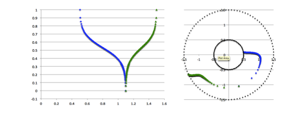
As shown by the following figure montage, this <math>~f(\varpi)</math> function very closely resembles the one generated by Imamura via a linear stability analysis.
|
PRACTICAL IMPLEMENTATION: At the two limits, <math>~\varpi = r_-</math> and <math>~\varpi = r_+</math>, the function, <math>~f(\varpi) \rightarrow +\infty</math>; while, at the limit, <math>~\varpi = r_\mathrm{mid}</math>, the function, <math>~f(\varpi) \rightarrow -\infty</math>. In practice we stay half of a radial zone away from these three limiting radial boundaries, so that the maximum and minimum values of <math>~f(\varpi)</math> are finite; then we strategically employ the finite values of the function at these near-boundary limits to rescale the function such that, in the plot shown below, it lies between zero (minimum amplitude) and unity (maximum amplitude). |
Now, the following general relation holds:
|
<math>~\tanh^{-1}x</math> |
<math>~=</math> |
<math>~\frac{1}{2} \ln\biggl( \frac{1+x}{1-x} \biggr) </math> |
for |
<math>x^2 < 1 \, .</math> |
Hence, for the innermost region of the toroidal configuration, we can set,
|
<math>~x</math> |
<math>~=</math> |
<math>~1 - 2 \biggl( \frac{\varpi - r_-}{r_\mathrm{mid}-r_-} \biggr) </math> |
|
<math>~\Rightarrow ~~~~ \frac{1+x}{1-x}</math> |
<math>~=</math> |
<math> ~\biggl[2 - 2 \biggl( \frac{\varpi - r_-}{r_\mathrm{mid}-r_-} \biggr)\biggr] \biggl[2 \biggl( \frac{\varpi - r_-}{r_\mathrm{mid}-r_-} \biggr)\biggr]^{-1} </math> |
|
|
<math>~=</math> |
<math> ~[(r_\mathrm{mid}-r_-) - ( \varpi - r_-)] [(\varpi - r_-)]^{-1} </math> |
|
|
<math>~=</math> |
<math> ~\frac{r_\mathrm{mid} - \varpi}{\varpi - r_-} \, . </math> |
Therefore we can write,
|
<math>~f(\varpi)</math> |
<math>~=</math> |
<math>~\frac{1}{2} \ln\biggl( \frac{r_\mathrm{mid} - \varpi}{\varpi - r_-} \biggr) </math> |
for |
<math>r_- < \varpi < r_\mathrm{mid} \, ;</math> |
and, similarly, we find,
|
<math>~f(\varpi)</math> |
<math>~=</math> |
<math>~\frac{1}{2} \ln\biggl( \frac{r_\mathrm{mid} - \varpi}{\varpi - r_+} \biggr) </math> |
for |
<math>r_\mathrm{mid} < \varpi < r_+ \, .</math> |
Now let's work on the phase function, <math>~\phi_m(\varpi)</math>, for the specific case, <math>~m=1</math>.
|
<math>~D(\varpi)</math> |
<math>~=</math> |
<math>~\frac{f(\varpi) - f_\mathrm{min}}{f_\mathrm{max} - f_\mathrm{min}} \, ;</math> |
|
<math>~\phi(\varpi) + \phi_0</math> |
<math>~=</math> |
<math>~\biggl\{\tan^{-1}[8\cdot D(\varpi)] - \frac{\pi}{2} \biggr\} + \frac{\pi}{10} \, .</math> |
Now, for the specific case being graphically illustrated here, <math>~f_\mathrm{min} = -2.99448</math> and <math>~f_\mathrm{max} = 2.64665</math>. Hence,
|
<math>~\phi(\varpi) + \frac{\pi}{2} </math> |
<math>~=</math> |
<math>~\tan^{-1}\biggl[8\cdot \biggl(\frac{f(\varpi) - f_\mathrm{min}}{f_\mathrm{max} - f_\mathrm{min}} \biggr)\biggr] </math> |
|
|
<math>~=</math> |
<math>~\tan^{-1}[a\cdot f(\varpi) + b] \, , </math> |
where, <math>~a = 1.41816</math> and <math>~b = 4.24664</math>.
See Also

|
|---|
|
© 2014 - 2021 by Joel E. Tohline |


