Difference between revisions of "User:Tohline/Appendix/Ramblings/Azimuthal Distortions"
(→Adopted Notation: Insert figure that compares with Imamura) |
(Begin showing empirically derived and analytically defined eigenvector) |
||
| Line 155: | Line 155: | ||
</div> | </div> | ||
whose relative amplitude — with a radial structure as specified inside the curly braces — is undergoing a uniform exponential growth but is otherwise unchanging. | whose relative amplitude — with a radial structure as specified inside the curly braces — is undergoing a uniform exponential growth but is otherwise unchanging. | ||
==Empirical Construction of Eigenvector== | |||
| Line 173: | Line 175: | ||
</div> | </div> | ||
First, specify a "midway" radial location, <math>~r_- < r_\mathrm{mid} < r_+ \, ,</math> at which the density fluctuation is smallest. Then define a function of the form, | |||
<div align="center"> | |||
<table border="0" cellpadding="5" align="center"> | |||
<tr> | |||
<td align="right"> | |||
<math>~f(\varpi)</math> | |||
</td> | |||
<td align="center"> | |||
<math>~=</math> | |||
</td> | |||
<td align="left"> | |||
<math>~\tanh^{-1}\biggl[1 - 2 \biggl( \frac{\varpi - r_-}{r_\mathrm{mid}-r_-} \biggr) \biggr]</math> | |||
</td> | |||
<td align="center"> | |||
for | |||
</td> | |||
<td align="left"> | |||
<math>r_- < \varpi < r_\mathrm{mid} \, ;</math> | |||
</td> | |||
</tr> | |||
<tr><td colspan="5" align="center">and</td></tr> | |||
<tr> | |||
<td align="right"> | |||
<math>~f(\varpi)</math> | |||
</td> | |||
<td align="center"> | |||
<math>~=</math> | |||
</td> | |||
<td align="left"> | |||
<math>~\tanh^{-1}\biggl[1 - 2 \biggl( \frac{\varpi - r_+}{r_\mathrm{mid}-r_+} \biggr) \biggr]</math> | |||
</td> | |||
<td align="center"> | |||
for | |||
</td> | |||
<td align="left"> | |||
<math>r_\mathrm{mid} < \varpi < r_+ \, .</math> | |||
</td> | |||
</tr> | |||
</table> | |||
</div> | |||
As shown by the following figure montage, this <math>~f(\varpi)</math> function very closely resembles the one generated by Imamura via a linear stability analysis. | |||
<div align="center"> | |||
<table border="1" cellpadding="10" width="50%"> | |||
<tr><td align="left"> | |||
'''<font color="maroon">PRACTICAL IMPLEMENTATION:</FONT>''' At the two limits, <math>~\varpi = r_-</math> and <math>~\varpi = r_+</math>, the function, <math>~f(\varpi) \rightarrow +\infty</math>; while, at the limit, <math>~\varpi = r_\mathrm{mid}</math>, the function, <math>~f(\varpi) \rightarrow -\infty</math>. In practice we stay ''half of a radial zone'' away from these three limiting radial boundaries, so that the maximum and minimum values of <math>~f(\varpi)</math> are finite; then we strategically employ the finite values of the function at these near-boundary limits to rescale the function such that, in the plot shown below, it lies between zero (minimum amplitude) and unity (maximum amplitude). | |||
</td></tr> | |||
</table> | |||
</div> | |||
<div align="center"> | <div align="center"> | ||
Revision as of 03:07, 5 January 2016
Analyzing Azimuthal Distortions

|
|---|
| | Tiled Menu | Tables of Content | Banner Video | Tohline Home Page | |
Adopted Notation
We will adopt the notation of J. E. Tohline & I. Hachisu (1988, ApJ, 361, 394). Specifically, drawing on their equation (2) but ignoring variations in the vertical coordinate, the mass density is given by the expression,
|
<math>~\rho</math> |
<math>~=</math> |
<math>~\rho_0 \biggl[ 1 + f(\varpi)e^{-i(\omega t - m\phi)} \biggr] \, ,</math> |
where it is understood that <math>~\rho_0</math>, which defines the structure of the initial axisymmetric equilibrium configuration, is generally a function of the cylindrical radial coordinate, <math>~\varpi</math>.
Using the subscript, <math>~m</math>, to identify the time-invariant coefficients and functions that characterize the intrinsic eigenvector of each azimuthal eigen-mode, and acknowledging that the associated eigenfrequency will in general be imaginary, that is,
|
<math>~\omega_m</math> |
<math>~=</math> |
<math>~\omega_R + i\omega_I \, ,</math> |
we expect each unstable mode to display the following behavior:
|
<math>~\biggl[ \frac{\rho}{\rho_0} - 1 \biggr]</math> |
<math>~=</math> |
<math>~f_m(\varpi)e^{-i[\omega_R t + i \omega_I t - m\phi_m(\varpi)]} </math> |
|
|
<math>~=</math> |
<math>~\biggl\{ f_m(\varpi)e^{-im\phi_m(\varpi)}\biggr\} e^{-i\omega_R t } \cdot e^{\omega_I t} </math> |
|
|
<math>~=</math> |
<math>~\biggl\{ f_m(\varpi)e^{-i[\omega_R t + m\phi_m(\varpi)]} \biggr\} e^{\omega_I t} \, .</math> |
Adopting Kojima's (1986) notation, that is, defining,
|
<math>~y_1 \equiv \frac{\omega_R}{\Omega_0} - m</math> |
and |
<math>~y_2 \equiv \frac{\omega_I}{\Omega_0} \, ,</math> |
the eigenvector's behavior can furthermore be described by the expression,
|
<math>~\biggl[ \frac{\rho}{\rho_0} - 1 \biggr]</math> |
<math>~=</math> |
<math>~\biggl\{ f_m(\varpi)e^{-i[(y_1+m) (\Omega_0 t) + m\phi_m(\varpi)]} \biggr\} e^{y_2 (\Omega_0 t)} </math> |
|
|
<math>~=</math> |
<math>~\biggl\{ f_m(\varpi)e^{-im[(y_1/m+1) (\Omega_0 t) + \phi_m(\varpi)]} \biggr\} e^{y_2 (\Omega_0 t)} \, .</math> |
Note that, as viewed from a frame of reference that is rotating with the mode pattern frequency,
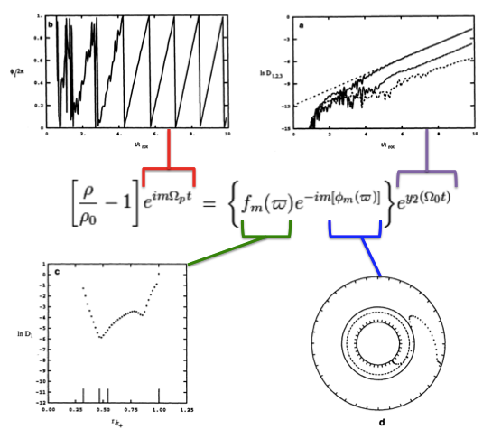
<math>\Omega_p \equiv \frac{\omega_R}{m} = \Omega_0\biggl(\frac{y_1}{m}+1\biggr) \, ,</math>
we should find an eigenvector of the form,
|
<math>~\biggl[ \frac{\rho}{\rho_0} - 1 \biggr]_\mathrm{rot} \equiv \biggl[ \frac{\rho}{\rho_0} - 1 \biggr]e^{im\Omega_p t}</math> |
<math>~=</math> |
<math>~\biggl\{ f_m(\varpi)e^{-im[\phi_m(\varpi)]} \biggr\} e^{y_2 (\Omega_0 t)} \, ,</math> |
whose relative amplitude — with a radial structure as specified inside the curly braces — is undergoing a uniform exponential growth but is otherwise unchanging.
Empirical Construction of Eigenvector
|
Four panels from figure 2 extracted† from p. 252 of J. W. Woodward, J. E. Tohline & I. Hachisu (1994)
"The Stability of Thick, Self-gravitating Disks in Protostellar Systems"
ApJ, vol. 420, pp. 247-267 © American Astronomical Society |
| †As displayed here, the layout of figure panels (a, b, c, d) has been modified from the original publication layout; otherwise, each panel is unmodified. |
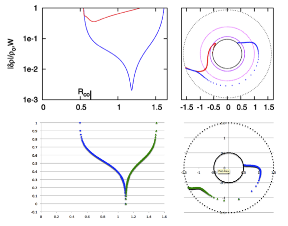
First, specify a "midway" radial location, <math>~r_- < r_\mathrm{mid} < r_+ \, ,</math> at which the density fluctuation is smallest. Then define a function of the form,
|
<math>~f(\varpi)</math> |
<math>~=</math> |
<math>~\tanh^{-1}\biggl[1 - 2 \biggl( \frac{\varpi - r_-}{r_\mathrm{mid}-r_-} \biggr) \biggr]</math> |
for |
<math>r_- < \varpi < r_\mathrm{mid} \, ;</math> |
| and | ||||
|
<math>~f(\varpi)</math> |
<math>~=</math> |
<math>~\tanh^{-1}\biggl[1 - 2 \biggl( \frac{\varpi - r_+}{r_\mathrm{mid}-r_+} \biggr) \biggr]</math> |
for |
<math>r_\mathrm{mid} < \varpi < r_+ \, .</math> |
As shown by the following figure montage, this <math>~f(\varpi)</math> function very closely resembles the one generated by Imamura via a linear stability analysis.
|
PRACTICAL IMPLEMENTATION: At the two limits, <math>~\varpi = r_-</math> and <math>~\varpi = r_+</math>, the function, <math>~f(\varpi) \rightarrow +\infty</math>; while, at the limit, <math>~\varpi = r_\mathrm{mid}</math>, the function, <math>~f(\varpi) \rightarrow -\infty</math>. In practice we stay half of a radial zone away from these three limiting radial boundaries, so that the maximum and minimum values of <math>~f(\varpi)</math> are finite; then we strategically employ the finite values of the function at these near-boundary limits to rescale the function such that, in the plot shown below, it lies between zero (minimum amplitude) and unity (maximum amplitude). |
See Also

|
|---|
|
© 2014 - 2021 by Joel E. Tohline |

