Difference between revisions of "User:Tohline/Appendix/Ramblings/ForOuShangli"
| (14 intermediate revisions by the same user not shown) | |||
| Line 5: | Line 5: | ||
{{LSU_HBook_header}} | {{LSU_HBook_header}} | ||
In order to download any one of the COLLADA-based files referenced below, go to [http://phys.lsu.edu/tohline/COLLADA/ http://phys.lsu.edu/tohline/COLLADA/index.html]. | In order to download any one of (a selected subset of) the COLLADA-based model files referenced below, go to [http://phys.lsu.edu/tohline/COLLADA/ http://phys.lsu.edu/tohline/COLLADA/index.html]. | ||
<table border="3" align="center" cellpadding="10"><tr><td align="center" bgcolor="red"> | |||
<table border="0" cellpadding="8" align="center"> | |||
<tr> | |||
<td align="center"> | |||
<font color="red">[http://phys.lsu.edu/tohline/COLLADA/index.html DOWNLOADABLE 3D MODELS]</font> | |||
</td> | |||
</tr> | |||
</table> | |||
</td></tr></table> | |||
==EFE Diagram (Review)== | ==EFE Diagram (Review)== | ||
| Line 24: | Line 34: | ||
==Example 3D Interactive Animations== | ==Example 3D Interactive Animations== | ||
For details, see the [[User:Tohline/ThreeDimensionalConfigurations/MeetsCOLLADAandOculusRiftS#The_COLLADA_Code_.26_Initial_3D_Scene|accompanying chapter titled, "Riemann Meets COLLADA & Oculus Rift S"]]. | For each model described below, note that, | ||
<table border="0" cellpadding="5" align="center"> | |||
<tr> | |||
<td align="right"> | |||
<math>~f \equiv \frac{\zeta_\mathrm{EFE}}{\Omega_\mathrm{EFE}}</math> | |||
</td> | |||
<td align="center"> | |||
<math>~=</math> | |||
</td> | |||
<td align="left"> | |||
<math>~- \frac{\lambda_\mathrm{EFE}}{\Omega_\mathrm{EFE}} \biggl[ \frac{1+(b/a)^2}{b/a} \biggr] \, .</math> | |||
</td> | |||
</tr> | |||
</table> | |||
For additional details, see the [[User:Tohline/ThreeDimensionalConfigurations/MeetsCOLLADAandOculusRiftS#The_COLLADA_Code_.26_Initial_3D_Scene|accompanying chapter titled, "Riemann Meets COLLADA & Oculus Rift S"]]. | |||
===b41c385=== | ===b41c385=== | ||
| Line 169: | Line 195: | ||
<td align="center"> | <td align="center"> | ||
<math>~f = + 4.061607 </math> | <math>~f = + 4.061607 </math> | ||
</td> | </td> | ||
</tr> | </tr> | ||
| Line 534: | Line 546: | ||
==Lenovo== | ==Lenovo== | ||
===COLLADA_to_gltf/COLLADA2GLTF-v2=== | ===KhronosGroup's COLLADA_to_gltf/COLLADA2GLTF-v2=== | ||
<ul> | |||
<li> | |||
ModelsB41C385<br /> | |||
Fundamentally this model is identical to the one developed earlier (and [[#b41c385|presented above]]) that shows how the ''DIRECT'' flow version of model "b41c385" appears when viewed from either the inertial or rotating reference frame: The ellipsoidal surface is purple [either translucent or opaque, as indicated]; the equatorial plane is identified by a series of small yellow markers; and 9 red markers depict the (slow, retrograde) Lagrangian motion of fluid elements that lie in the equatorial plane. | |||
<ul> | |||
<li> | |||
<font color="maroon">MultiFluidElements/MultiLagrange26.dae</font> [translucent purple] (05/28/2020) and <font color="orange">/output/MultiLagrange26.glb</font> (06/04/2020) — both files also copied (01/31/2021) to LSU physics website with filename … COLLADA/b41c385DirRotating. | |||
<table border="1" cellpadding="8" align="center" width="50%"><tr><td align="left"> | |||
<div align="center"><math>~b/a = 0.41~~~~~c/a = 0.385</math><br />'''<font color="red">DIRECT</font>''' flow - as viewed from '''<font color="red">ROTATING</font>''' frame</div> | |||
</td></tr></table> | |||
</li> | |||
</ul> | |||
<ul> | |||
<li> | |||
<font color="maroon">InertialFrame/Inertial34.dae</font> [opaque purple] (05/29/2020) and <font color="orange">/output/Inertial34.glb</font> (06/04/2020) — both files also copied (01/31/2021) to LSU physics website with filename … COLLADA/b41c385DirInertial. | |||
<table border="1" cellpadding="8" align="center" width="50%"><tr><td align="left"> | |||
<div align="center"><math>~b/a = 0.41~~~~~c/a = 0.385</math><br />'''<font color="red">DIRECT</font>''' flow - as viewed from '''<font color="red">INERTIAL</font>''' frame</div> | |||
</td></tr></table> | |||
</li> | |||
</ul> | |||
</li> | |||
</ul> | |||
<ul> | <ul> | ||
<li> | <li> | ||
ModelsB90C333<br /> | ModelsB90C333<br /> | ||
Fundamentally this model is identical to the one developed earlier (and [[#b90c333|presented above]]) that shows how the ''DIRECT'' flow version of model "b90c333" appears when viewed from the inertial reference frame: The ellipsoidal surface is translucent | Fundamentally this model is identical to the one developed earlier (and [[#b90c333|presented above]]) that shows how the ''DIRECT'' flow version of model "b90c333" appears when viewed from either the inertial or a rotating reference frame: The ellipsoidal surface is purple [either translucent or opaque, as indicated]; the equatorial plane is identified by a series of small yellow markers; and 9 red markers depict the (slow, prograde) Lagrangian motion of fluid elements that lie in the equatorial plane. | ||
<ul> | <ul> | ||
<li> | <li> | ||
<font color="maroon"> | <font color="maroon">FastRot79.dae</font> [translucent purple] (06/03/2020) and <font color="orange">/output/FastRot79.glb</font> (06/04/2020) — both files also copied (01/31/2021) to LSU physics website with filename … COLLADA/b90c333DirRotating. | ||
<table border="1" cellpadding="8" align="center" width="50%"><tr><td align="left"> | <table border="1" cellpadding="8" align="center" width="50%"><tr><td align="left"> | ||
<div align="center"><math>~b/a = 0.90~~~~~c/a = 0.333</math><br />'''<font color="red">DIRECT</font>''' flow - as viewed from '''<font color="red">ROTATING</font>''' frame</div> | <div align="center"><math>~b/a = 0.90~~~~~c/a = 0.333</math><br />'''<font color="red">DIRECT</font>''' flow - as viewed from '''<font color="red">ROTATING</font>''' frame</div> | ||
</td></tr></table> | |||
</li> | |||
</ul> | |||
<ul> | |||
<li> | |||
<font color="maroon">FastInertial80.dae</font> [opaque purple] (06/03/2020) — Also available is <font color="orange">../output/FastInertial80.glb</font> (06/04/2020) — both files also copied (01/31/2021) to LSU physics website with filename … COLLADA/b90c333DirInertial. | |||
<table border="1" cellpadding="8" align="center" width="50%"><tr><td align="left"> | |||
<div align="center"><math>~b/a = 0.90~~~~~c/a = 0.333</math><br />'''<font color="red">DIRECT</font>''' flow - as viewed from '''<font color="red">INERTIAL</font>''' frame</div> | |||
</td></tr></table> | </td></tr></table> | ||
</li> | </li> | ||
| Line 558: | Line 597: | ||
<ul> | <ul> | ||
<li> | <li> | ||
ModelsB74C692<br /> | |||
Fundamentally this model is identical to the one developed earlier (and [[# | Fundamentally this model is identical to the one developed earlier (and [[#b74c692|presented above]]) that shows how the ''DIRECT'' flow version of model "b74c692" appears when viewed from the rotating reference frame: The ellipsoidal surface is translucent (purple); the equatorial plane is identified by a series of small yellow markers; and 9 red markers depict the (slow, retrograde) Lagrangian motion of fluid elements that lie in the equatorial plane. | ||
<ul> | |||
<li> | |||
<font color="maroon">TestMulti74.dae</font> (06/03/2020) — Also available is <font color="orange">../output/TestMulti74.glb</font> (06/02/2020) | |||
<table border="1" cellpadding="8" align="center" width="50%"><tr><td align="left"> | |||
<div align="center"><math>~b/a = 0.74~~~~~c/a = 0.692</math><br />'''<font color="red">DIRECT</font>''' flow - as viewed from '''<font color="red">ROTATING</font>''' frame</div> | |||
</td></tr></table> | |||
</li> | |||
</ul> | |||
<ul> | |||
<li> | |||
<font color="maroon">InertialB74C692aa.dae</font> [opaque purple] (06/02/2020) | |||
<table border="1" cellpadding="8" align="center" width="50%"><tr><td align="left"> | |||
<div align="center"><math>~b/a = 0.74~~~~~c/a = 0.692</math><br />'''<font color="red">DIRECT</font>''' flow - as viewed from '''<font color="red">INERTIAL</font>''' frame</div> | |||
</td></tr></table> | |||
</li> | |||
</ul> | |||
</li> | |||
</ul> | |||
<ul> | |||
<li> | |||
(no subdirectory)<br /> | |||
Fundamentally this model is identical to the one developed earlier (and [[#b28c256|presented above]]) that shows how the ''DIRECT'' flow version of model "b28c256" appears when viewed from the inertial reference frame: The ellipsoidal surface is purple [either translucent or opaque, as indicated]; the equatorial plane is identified by a series of small yellow markers; and 9 red markers depict the (very slow, retrograde) Lagrangian motion of fluid elements that lie in the equatorial plane. | |||
<ul> | |||
<li> | |||
<font color="maroon">Pencil94.dae</font> [translucent purple surface] (06/04/2020) and <font color="orange">/output/Pencil94.glb</font> (06/04/2020) — both files also copied (01/30/2021) to LSU physics website with filename … COLLADA/b28c256DirRotating. | |||
<table border="1" cellpadding="8" align="center" width="50%"><tr><td align="left"> | |||
<div align="center"><math>~b/a = 0.28~~~~~c/a = 0.256</math><br />'''<font color="red">DIRECT</font>''' flow - as viewed from '''<font color="red">ROTATING</font>''' frame</div> | |||
</td></tr></table> | |||
</li> | |||
</ul> | |||
<ul> | <ul> | ||
<li> | <li> | ||
<font color="maroon"> | <font color="maroon">PencilInertial96.dae</font> [opaque purple surface] (06/04/2020) and <font color="orange">/output/PencilInertial95.glb</font> (06/04/2020) — both files also copied (01/30/2021) to LSU physics website with filename … COLLADA/b28c256DirInertial. | ||
<table border="1" cellpadding="8" align="center" width="50%"><tr><td align="left"> | <table border="1" cellpadding="8" align="center" width="50%"><tr><td align="left"> | ||
<div align="center"><math>~b/a = 0. | <div align="center"><math>~b/a = 0.28~~~~~c/a = 0.256</math><br />'''<font color="red">DIRECT</font>''' flow - as viewed from '''<font color="red">INERTIAL</font>''' frame</div> | ||
</td></tr></table> | </td></tr></table> | ||
</li> | </li> | ||
Latest revision as of 21:50, 31 January 2021
For Shangli Ou

|
|---|
| | Tiled Menu | Tables of Content | Banner Video | Tohline Home Page | |
In order to download any one of (a selected subset of) the COLLADA-based model files referenced below, go to http://phys.lsu.edu/tohline/COLLADA/index.html.
|
|
EFE Diagram (Review)
| Figure 1 |
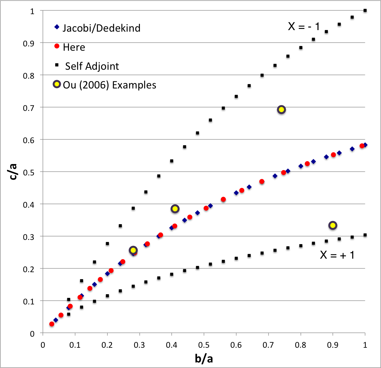
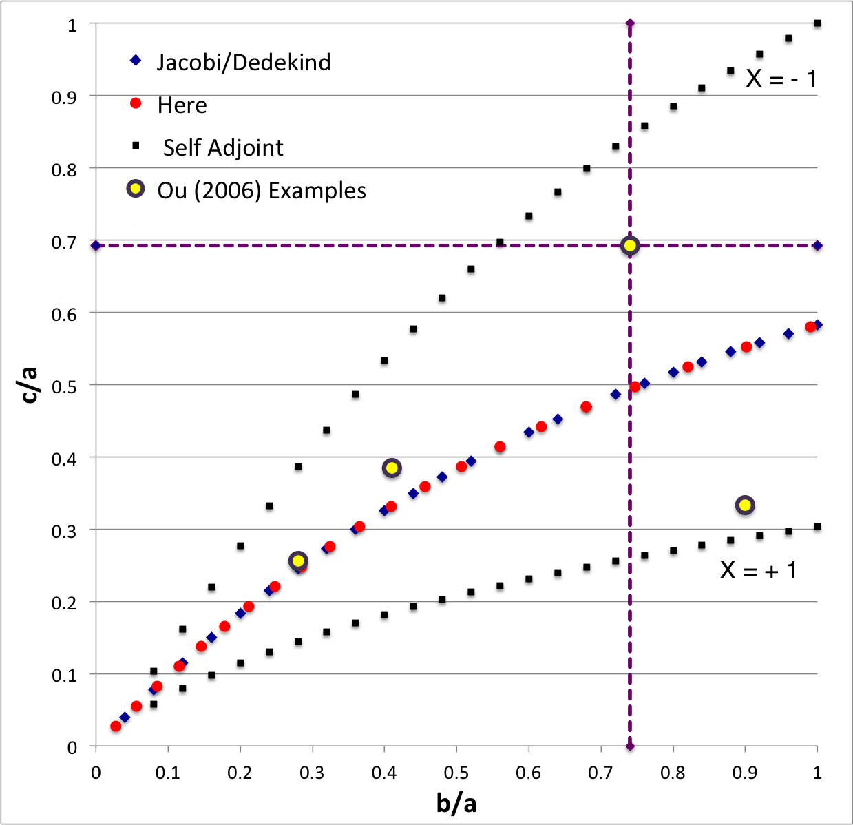
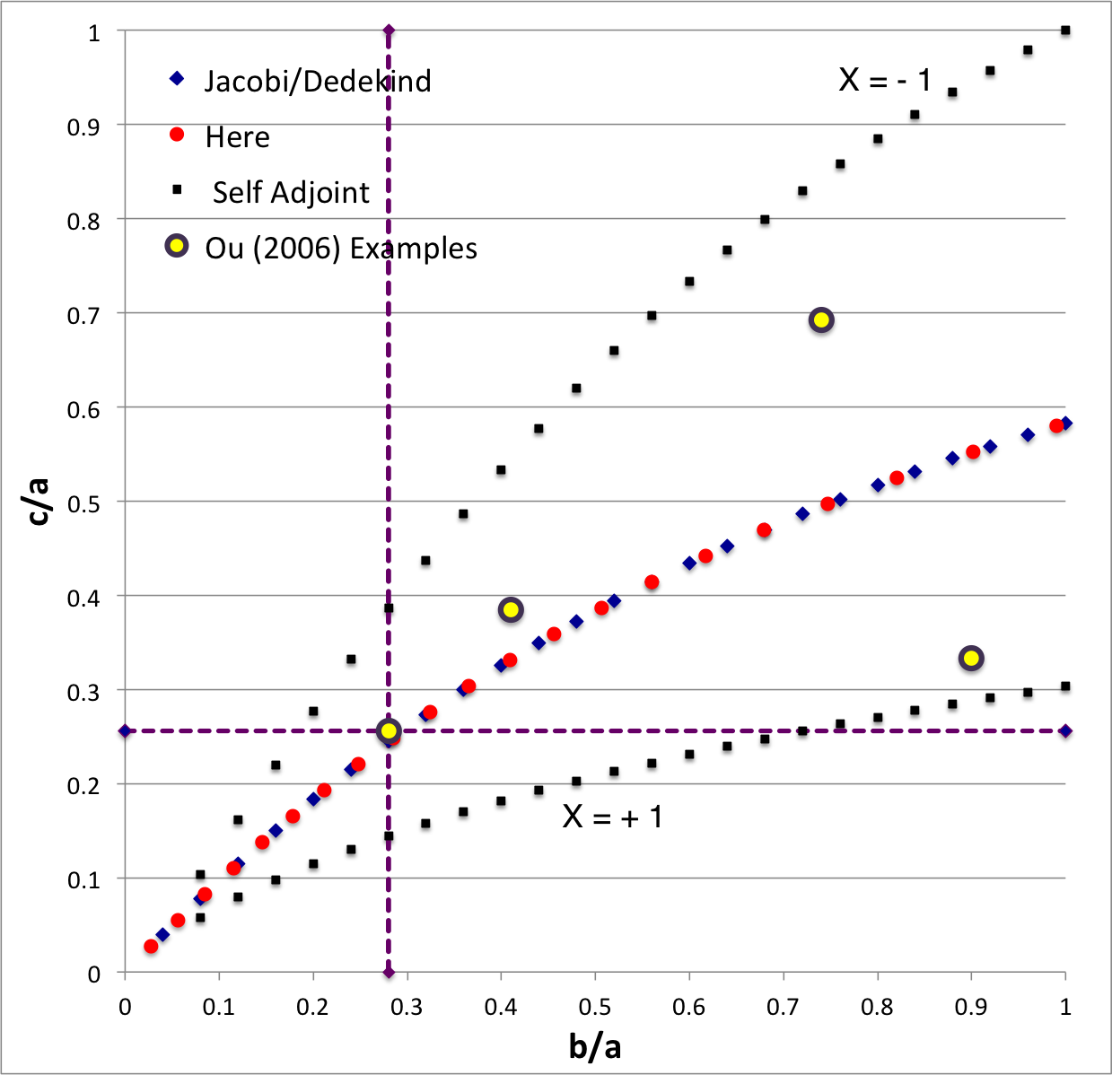
In the context of our broad discussion of ellipsoidal figures of equilibrium, the label "EFE Diagram" refers to a two-dimensional parameter space defined by the pair of axis ratios (b/a, c/a), usually covering the ranges, 0 ≤ b/a ≤ 1 and 0 ≤ c/a ≤ 1. The classic/original version of this diagram appears as Figure 2 on p. 902 of S. Chandrasekhar (1965, ApJ, vol. 142, pp. 890-921); a somewhat less cluttered version appears on p. 147 of Chandrasekhar's [EFE].
The version of the EFE Diagram shown here, on the left, highlights four model sequences, all of which also can be found in the original version:
- Jacobi sequence — the smooth curve that runs through the set of small, dark-blue, diamond-shaped markers; the data identifying the location of these markers have been drawn from §39, Table IV of [EFE]. The small red circular markers lie along this same sequence; their locations are taken from our own determinations, as detailed in Table 2 of our accompanying discussion of Jacobi ellipsoids. All of the models along this sequence have <math>~f \equiv \zeta/\Omega_f = 0</math> and are therefore solid-body rotators, that is, there is no internal motion when the configuration is viewed from a frame that is rotating with frequency, <math>~\Omega_f</math>.
- Dedekind sequence — a smooth curve that lies precisely on top of the Jacobi sequence. Each configuration along this sequence is adjoint to a model on the Jacobi sequence that shares its (b/a, c/a) axis-ratio pair. All ellipsoidal figures along this sequence have <math>~1/f = \Omega_f/\zeta = 0</math> and are therefore stationary as viewed from the inertial frame; the angular momentum of each configuration is stored in its internal motion (vorticity).
- The X = -1 self-adjoint sequence — At every point along this sequence, the value of the key frequency ratio, <math>~\zeta/\Omega_f</math>, in the adjoint configuration <math>~(f_+)</math> is identical to the value of the frequency ratio in the direct configuration <math>~(f_-)</math>; specifically, <math>~f_+ = f_- = -(a^2+b^2)/(ab)</math>. The data identifying the location of the small, solid-black markers along this sequence have been drawn from §48, Table VI of [EFE].
- The X = +1 self-adjoint sequence — At every point along this sequence, the value of the key frequency ratio, <math>~\zeta/\Omega_f</math>, in the adjoint configuration <math>~(f_+)</math> is identical to the value of the frequency ratio in the direct configuration <math>~(f_-)</math>; specifically, <math>~f_+ = f_- = +(a^2+b^2)/(ab)</math>. The data identifying the location of the small, solid-black markers along this sequence have been drawn from §48, Table VI of [EFE].
Riemann S-type ellipsoids all lie between or on the two (self-adjoint) curves marked "X = -1" and "X = +1" in the EFE Diagram. The yellow circular markers in the diagram shown here, on the left, identify four Riemann S-type ellipsoids that were examined by Ou (2006) and that we have also chosen to use as examples.
Example 3D Interactive Animations
For each model described below, note that,
|
<math>~f \equiv \frac{\zeta_\mathrm{EFE}}{\Omega_\mathrm{EFE}}</math> |
<math>~=</math> |
<math>~- \frac{\lambda_\mathrm{EFE}}{\Omega_\mathrm{EFE}} \biggl[ \frac{1+(b/a)^2}{b/a} \biggr] \, .</math> |
For additional details, see the accompanying chapter titled, "Riemann Meets COLLADA & Oculus Rift S".
b41c385
The model that we have chosen to use in our first successful construction of a COLLADA-based, 3D and interactive animation has the following properties; this model has been selected from Table 2 of our accompanying discussion of Riemann S-type ellipsoids:
|
|
<math>~\frac{b}{a} = 0.41</math> |
|
||||
|
<math>~\frac{c}{a} = 0.385</math> |
||||||
|
Direct |
|
Adjoint |
||||
|
<math>~\Omega_\mathrm{EFE} = 0.547874</math> |
<math>~\Omega_\mathrm{EFE} = - 0.079886</math> |
|||||
|
<math>~\lambda_\mathrm{EFE} = 0.079886</math> |
<math>~\lambda_\mathrm{EFE} = - 0.547874</math> |
|||||
|
<math>~f = - 0.415418</math> |
<math>~f = - 19.53923</math> |
|||||
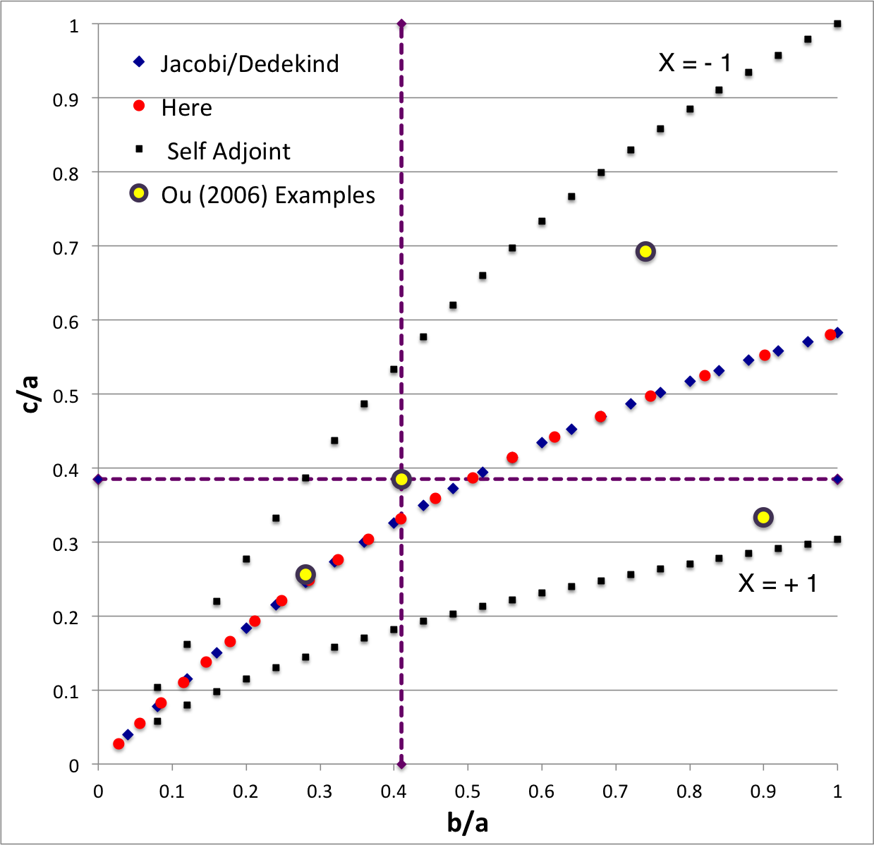
The subscript "EFE" on Ω and λ means that the relevant frequency is given in units that have been adopted in [EFE], that is, in units of <math>~[\pi G\rho]^{1 / 2}</math>. In Figure 2a, the yellow circular marker, that has been placed where the pair of purple dashed lines cross, identifies the location of this model in the "c/a versus b/a" EFE Diagram that appears as Figure 2 on p. 902 of S. Chandrasekhar (1965); essentially the same diagram appears in §49 (p. 147) of [EFE].
In a separate chapter we have discussed various properties of uniformly rotating, Jacobi ellipsoids; they are equilibrium configurations that lie along the sequence that runs from "M2" (on the b/a = 1, Maclaurin sequence) to the origin of this diagram. Our chosen model lies off of — just above — the Jacobi-ellipsoid sequence, which means that it is not rotating as a solid body. Instead, as we focus first on the direct (as opposed to the adjoint) configuration, we appreciate that while the ellipsoid is spinning prograde (counter-clockwise) with a frequency given by |ΩEFE|, each Lagrangian fluid element inside as well as on the surface of the ellipsoid is traveling retrograde (clockwise) along an elliptical path with a frequency given by |λEFE|.
b90c333
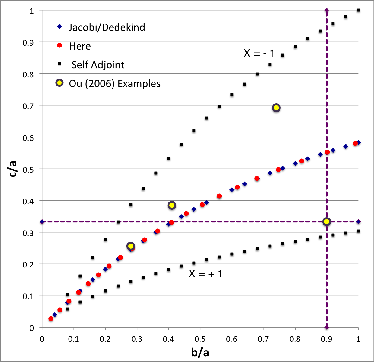
The model that we have chosen to use in our second successful construction of a COLLADA-based, 3D and interactive animation has the following properties; this model has been selected from Table 2 of our accompanying discussion of Riemann S-type ellipsoids:
|
|
<math>~\frac{b}{a} = 0.90</math> |
|
||||
|
<math>~\frac{c}{a} = 0.333</math> |
||||||
|
Direct |
|
Adjoint |
||||
|
<math>~\Omega_\mathrm{EFE} = 0.447158</math> |
<math>~\Omega_\mathrm{EFE} = 0.221411</math> |
|||||
|
<math>~\lambda_\mathrm{EFE} = - 0.221411</math> |
<math>~\lambda_\mathrm{EFE} = - 0.447158 </math> |
|||||
|
<math>~f = + 0.995805</math> |
<math>~f = + 4.061607 </math> |
|||||
b74c692
The model that we have chosen to use in our third successful construction of a COLLADA-based, 3D and interactive animation has the following properties; this model has been selected from Table 2 of our accompanying discussion of Riemann S-type ellipsoids:
|
|
<math>~\frac{b}{a} = 0.74</math> |
|
||||
|
<math>~\frac{c}{a} = 0.692</math> |
||||||
|
Direct |
|
Adjoint |
||||
|
<math>~\Omega_\mathrm{EFE} = 0.638747</math> |
<math>~\Omega_\mathrm{EFE} = - 0.217773</math> |
|||||
|
<math>~\lambda_\mathrm{EFE} = 0.217773</math> |
<math>~\lambda_\mathrm{EFE} = - 0.638747 </math> |
|||||
|
<math>~f = - 0.713019</math> |
<math>~f = - 6.13413 </math> |
|||||
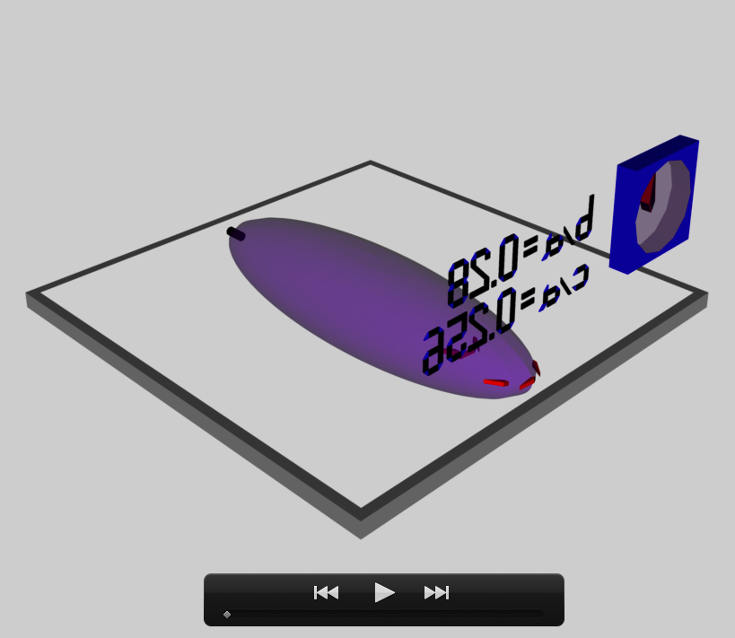
b28c256
The model that we have chosen to use in our second successful construction of a COLLADA-based, 3D and interactive animation has the following properties; this model has been selected from Table 2 of our accompanying discussion of Riemann S-type ellipsoids:
|
|
<math>~\frac{b}{a} = 0.28</math> |
|
||||
|
<math>~\frac{c}{a} = 0.256</math> |
||||||
|
Direct |
|
Adjoint |
||||
|
<math>~\Omega_\mathrm{EFE} = 0.456676</math> |
<math>~\Omega_\mathrm{EFE} = - 0.020692</math> |
|||||
|
<math>~\lambda_\mathrm{EFE} = 0.020692</math> |
<math>~\lambda_\mathrm{EFE} = - 0.456676</math> |
|||||
|
<math>~f = - 0.174510</math> |
<math>~f = - 85.0007</math> |
|||||
Catalog of Local 3D Model Files (cannot be downloaded)
3Dviewers
AutoRiemann
-
Trial.Ou_b28c256
Generally speaking ... Translucent surface; one Lagrangian (red surface arrow) fluid element; no axis arrow; NO WALL LABELs.-
Ou_b28c256.Dir.Inertial.dae (12/01/2019)
<math>~b/a = 0.28~~~~~c/a = 0.256</math>
DIRECT flow - as viewed from INERTIAL frame -
Ou_b28c256.Dir.Rot.dae (12/01/2019)
<math>~b/a = 0.28~~~~~c/a = 0.256</math>
DIRECT flow - as viewed from ROTATING frame -
Ou_b28c256.Adj.Inertial.dae (12/01/2019)
<math>~b/a = 0.28~~~~~c/a = 0.256</math>
ADJOINT flow - as viewed from INERTIAL frame -
Ou_b28c256.Adj.Rot.dae (12/01/2019)
<math>~b/a = 0.28~~~~~c/a = 0.256</math>
ADJOINT flow - as viewed from ROTATING frame
-
Ou_b28c256.Dir.Inertial.dae (12/01/2019)
-
Cylinder
Generally speaking ... Translucent surface; one Lagrangian (red surface arrow) fluid element; no axis arrow; PROBLEM RESETING CLOCK.-
Dir.Inertial_b28c256.labeled.dae (12/22/2019)
<math>~b/a = 0.28~~~~~c/a = 0.256</math>
DIRECT flow - as viewed from INERTIAL frame -
Dir.Rot_b28c256.labeled.dae (12/22/2019)
<math>~b/a = 0.28~~~~~c/a = 0.256</math>
DIRECT flow - as viewed from ROTATING frame
-
Dir.Inertial_b28c256.labeled.dae (12/22/2019)
-
BESTmodels
Generally speaking ... Translucent surface; six Lagrangian (red arrow markers) fluid elements.-
b28c256/b28c256.DI.dae (01/02/2020)
<math>~b/a = 0.28~~~~~c/a = 0.256</math>
DIRECT flow - as viewed from INERTIAL frame -
b28c256/b28c256.DRot.dae (01/02/2020)
<math>~b/a = 0.28~~~~~c/a = 0.256</math>
DIRECT flow - as viewed from ROTATING frame -
b28c256/b28c256.AI.dae (01/02/2020)
<math>~b/a = 0.28~~~~~c/a = 0.256</math>
ADJOINT flow - as viewed from INERTIAL frame -
b28c256/b28c256.ARot.dae (01/02/2020)
<math>~b/a = 0.28~~~~~c/a = 0.256</math>
ADJOINT flow - as viewed from ROTATING frame -
b41c385/b41c385.DI.dae (01/02/2020)
<math>~b/a = 0.41~~~~~c/a = 0.385</math>
DIRECT flow - as viewed from INERTIAL frame -
b41c385/b41c385.DRot.dae (01/02/2020)
<math>~b/a = 0.41 ~~~~~c/a = 0.385</math>
DIRECT flow - as viewed from ROTATING frame -
b41c385/b41c385.AI.dae (01/02/2020)
<math>~b/a = 0.41 ~~~~~c/a = 0.385</math>
ADJOINT flow - as viewed from INERTIAL frame -
b41c385/b41c385.ARot.dae (01/02/2020)
<math>~b/a = 0.41 ~~~~~c/a = 0.385</math>
ADJOINT flow - as viewed from ROTATING frame -
b74c692/b74c692.DI.dae (01/02/2020)
<math>~b/a = 0.74~~~~~c/a = 0.692</math>
DIRECT flow - as viewed from INERTIAL frame -
b74c692/b74c692.DRot.dae (01/02/2020)
<math>~b/a = 0.74 ~~~~~c/a = 0.692 </math>
DIRECT flow - as viewed from ROTATING frame -
b74c692/b74c692.AI.dae (01/02/2020)
<math>~b/a = 0.74 ~~~~~c/a = 0.692 </math>
ADJOINT flow - as viewed from INERTIAL frame -
b74c692/b74c692.ARot.dae (01/02/2020)
<math>~b/a = 0.74 ~~~~~c/a = 0.692 </math>
ADJOINT flow - as viewed from ROTATING frame -
b90c333/b90c333.DI.dae (01/02/2020)
<math>~b/a = 0.90~~~~~c/a = 0.333</math>
DIRECT flow - as viewed from INERTIAL frame -
b90c333/b90c333.DRot.dae (01/02/2020)
<math>~b/a = 0.90 ~~~~~c/a = 0.333 </math>
DIRECT flow - as viewed from ROTATING frame -
b90c333/b90c333.AI.dae (01/02/2020)
<math>~b/a = 0.90 ~~~~~c/a = 0.333 </math>
ADJOINT flow - as viewed from INERTIAL frame -
b90c333/b90c333.ARot.dae (01/02/2020)
<math>~b/a = 0.90 ~~~~~c/a = 0.333 </math>
ADJOINT flow - as viewed from ROTATING frame
-
b28c256/b28c256.DI.dae (01/02/2020)
-
TypeI
Translucent surface; just Type I tilted figure motion (no Lagrangian fluid elements).-
TypeIa10.GREAT.dae (01/04/2020)
<math>~b/a = 1.25~~~~~c/a = 0.470</math>
DIRECT figure (only) motion - as viewed from INERTIAL frame
-
TypeIa10.GREAT.dae (01/04/2020)
-
TypeI/Lagrange
Depicts motion of (3) Lagrangian fluid elements across an opaque surface; no figure motion; three separate, tilted fluid orbits are identified by small yellow markers.-
TL15.lagrange.dae (01/26/2020)
<math>~b/a = 1.25~~~~~c/a = 0.470</math>
LAGRANGIAN element (only) motion - as viewed from ROTATING frame
-
TL15.lagrange.dae (01/26/2020)
Lenovo
KhronosGroup's COLLADA_to_gltf/COLLADA2GLTF-v2
-
ModelsB41C385
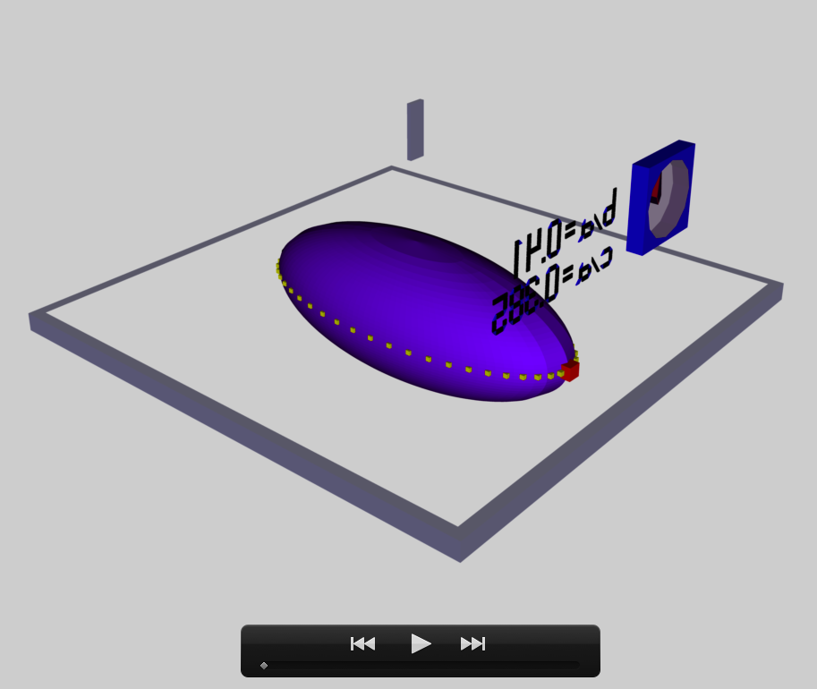
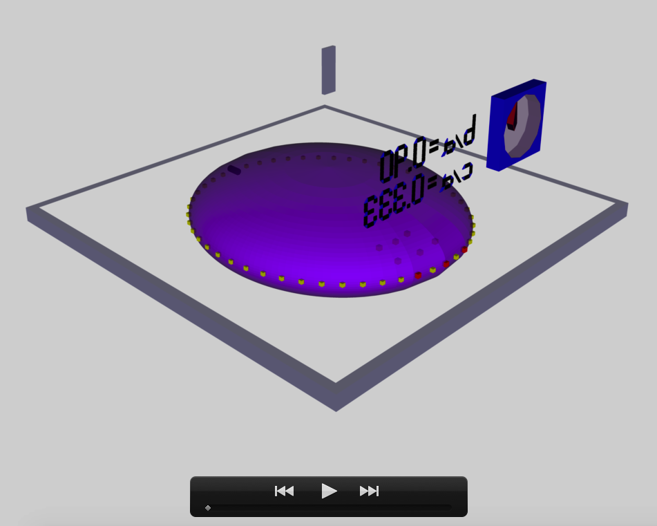
Fundamentally this model is identical to the one developed earlier (and presented above) that shows how the DIRECT flow version of model "b41c385" appears when viewed from either the inertial or rotating reference frame: The ellipsoidal surface is purple [either translucent or opaque, as indicated]; the equatorial plane is identified by a series of small yellow markers; and 9 red markers depict the (slow, retrograde) Lagrangian motion of fluid elements that lie in the equatorial plane.-
MultiFluidElements/MultiLagrange26.dae [translucent purple] (05/28/2020) and /output/MultiLagrange26.glb (06/04/2020) — both files also copied (01/31/2021) to LSU physics website with filename … COLLADA/b41c385DirRotating.
<math>~b/a = 0.41~~~~~c/a = 0.385</math>
DIRECT flow - as viewed from ROTATING frame
-
InertialFrame/Inertial34.dae [opaque purple] (05/29/2020) and /output/Inertial34.glb (06/04/2020) — both files also copied (01/31/2021) to LSU physics website with filename … COLLADA/b41c385DirInertial.
<math>~b/a = 0.41~~~~~c/a = 0.385</math>
DIRECT flow - as viewed from INERTIAL frame
-
MultiFluidElements/MultiLagrange26.dae [translucent purple] (05/28/2020) and /output/MultiLagrange26.glb (06/04/2020) — both files also copied (01/31/2021) to LSU physics website with filename … COLLADA/b41c385DirRotating.
-
ModelsB90C333
Fundamentally this model is identical to the one developed earlier (and presented above) that shows how the DIRECT flow version of model "b90c333" appears when viewed from either the inertial or a rotating reference frame: The ellipsoidal surface is purple [either translucent or opaque, as indicated]; the equatorial plane is identified by a series of small yellow markers; and 9 red markers depict the (slow, prograde) Lagrangian motion of fluid elements that lie in the equatorial plane.-
FastRot79.dae [translucent purple] (06/03/2020) and /output/FastRot79.glb (06/04/2020) — both files also copied (01/31/2021) to LSU physics website with filename … COLLADA/b90c333DirRotating.
<math>~b/a = 0.90~~~~~c/a = 0.333</math>
DIRECT flow - as viewed from ROTATING frame
-
FastInertial80.dae [opaque purple] (06/03/2020) — Also available is ../output/FastInertial80.glb (06/04/2020) — both files also copied (01/31/2021) to LSU physics website with filename … COLLADA/b90c333DirInertial.
<math>~b/a = 0.90~~~~~c/a = 0.333</math>
DIRECT flow - as viewed from INERTIAL frame
-
FastRot79.dae [translucent purple] (06/03/2020) and /output/FastRot79.glb (06/04/2020) — both files also copied (01/31/2021) to LSU physics website with filename … COLLADA/b90c333DirRotating.
-
ModelsB74C692
Fundamentally this model is identical to the one developed earlier (and presented above) that shows how the DIRECT flow version of model "b74c692" appears when viewed from the rotating reference frame: The ellipsoidal surface is translucent (purple); the equatorial plane is identified by a series of small yellow markers; and 9 red markers depict the (slow, retrograde) Lagrangian motion of fluid elements that lie in the equatorial plane.-
TestMulti74.dae (06/03/2020) — Also available is ../output/TestMulti74.glb (06/02/2020)
<math>~b/a = 0.74~~~~~c/a = 0.692</math>
DIRECT flow - as viewed from ROTATING frame
-
InertialB74C692aa.dae [opaque purple] (06/02/2020)
<math>~b/a = 0.74~~~~~c/a = 0.692</math>
DIRECT flow - as viewed from INERTIAL frame
-
TestMulti74.dae (06/03/2020) — Also available is ../output/TestMulti74.glb (06/02/2020)
-
(no subdirectory)
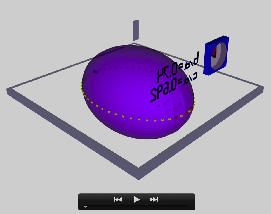
Fundamentally this model is identical to the one developed earlier (and presented above) that shows how the DIRECT flow version of model "b28c256" appears when viewed from the inertial reference frame: The ellipsoidal surface is purple [either translucent or opaque, as indicated]; the equatorial plane is identified by a series of small yellow markers; and 9 red markers depict the (very slow, retrograde) Lagrangian motion of fluid elements that lie in the equatorial plane.-
Pencil94.dae [translucent purple surface] (06/04/2020) and /output/Pencil94.glb (06/04/2020) — both files also copied (01/30/2021) to LSU physics website with filename … COLLADA/b28c256DirRotating.
<math>~b/a = 0.28~~~~~c/a = 0.256</math>
DIRECT flow - as viewed from ROTATING frame
-
PencilInertial96.dae [opaque purple surface] (06/04/2020) and /output/PencilInertial95.glb (06/04/2020) — both files also copied (01/30/2021) to LSU physics website with filename … COLLADA/b28c256DirInertial.
<math>~b/a = 0.28~~~~~c/a = 0.256</math>
DIRECT flow - as viewed from INERTIAL frame
-
Pencil94.dae [translucent purple surface] (06/04/2020) and /output/Pencil94.glb (06/04/2020) — both files also copied (01/30/2021) to LSU physics website with filename … COLLADA/b28c256DirRotating.
Workfolder
Wiki_edits
-
CoordinateSystems
Fundamentally this model is identical to the one developed earlier (and presented above) that shows how the DIRECT flow version of model "b41c385" appears when viewed from the inertial reference frame: The ellipsoidal surface is translucent (purple); the equatorial plane is identified by a series of small yellow markers; and a single, red marker depicts the (slow, retrograde) Lagrangian motion of one fluid element that lies in the equatorial plane. But here, in addition across the "northern" hemisphere of the ellipsoid, a sequence of small yellow markers is used to identify the location of one <math>~\lambda_3</math> coordinate curve as defined within our so-called "T8" coordinate system.-
Lambda3Curve03.dae (12/26/2020)
<math>~b/a = 0.41~~~~~c/a = 0.385</math>
DIRECT flow - as viewed from INERTIAL frame
-
Lambda3Curve03.dae (12/26/2020)
See Also
- Discussion of Ou's Riemann-Like Ellipsoids
- Riemann Meets COLLADA & Oculus Rift S: Example (b/a, c/a) = (0.41, 0.385)

|
|---|
|
© 2014 - 2021 by Joel E. Tohline |
