Difference between revisions of "User:Tohline/Apps/ImamuraHadleyCollaboration"
(→Plots of a Few Example Eigenvectors: Insert image of Model J1 amplitude) |
(→Setup) |
||
| (53 intermediate revisions by the same user not shown) | |||
| Line 3: | Line 3: | ||
=Characteristics of Unstable Eigenvectors in Self-Gravitating Tori= | =Characteristics of Unstable Eigenvectors in Self-Gravitating Tori= | ||
{{LSU_HBook_header}} | {{LSU_HBook_header}} | ||
Using numerical hydrodynamic techniques, the [[#See_Also|Imamura & Hadley collaboration]] — see especially [http://adsabs.harvard.edu/abs/2011Ap%26SS.334....1H Paper I] and [http://adsabs.harvard.edu/abs/2014Ap%26SS.353..191H Paper II] — has studied the dynamical development of nonaxisymmetric instabilities in toroidal configurations that have a range of "star-to-disk" mass ratios and a wide variety of (initially axisymmetric) geometric structures. Our principal aim, here, is to compare the results of these numerical investigations with what is known, analytically, about normal modes of oscillation and nonaxisymmetric instabilities in [[User:Tohline/Apps/PapaloizouPringleTori#Massless_Polytropic_Tori|''massless'' Papaloizou-Pringle tori]]. On the analytic side, our focus is on the very informative stability analysis published by [http://adsabs.harvard.edu/abs/1985MNRAS.216..553B Blaes (1985; hereafter, Blaes85)]. | |||
<!-- In what follows, we will draw heavily from three publications: (1) [http://adsabs.harvard.edu/abs/1990ApJ...361..394T J. E. Tohline & I. Hachisu (1990, ApJ, 361, 394-407)] — hereafter, TH90 — (2) [http://adsabs.harvard.edu/abs/1994ApJ...420..247W J. W. Woodward, J. E. Tohline, & I. Hachisu (1994, ApJ, 420, 247-267)] — hereafter, WTH94 — and (3) [http://adsabs.harvard.edu/abs/2011Ap%26SS.334....1H K. Hadley & J. N. Imamura (2011, ''Astrophysics and Space Science'', 334, 1)] — hereafter, HI11.--> | <!-- In what follows, we will draw heavily from three publications: (1) [http://adsabs.harvard.edu/abs/1990ApJ...361..394T J. E. Tohline & I. Hachisu (1990, ApJ, 361, 394-407)] — hereafter, TH90 — (2) [http://adsabs.harvard.edu/abs/1994ApJ...420..247W J. W. Woodward, J. E. Tohline, & I. Hachisu (1994, ApJ, 420, 247-267)] — hereafter, WTH94 — and (3) [http://adsabs.harvard.edu/abs/2011Ap%26SS.334....1H K. Hadley & J. N. Imamura (2011, ''Astrophysics and Space Science'', 334, 1)] — hereafter, HI11.--> | ||
As we [[User:Tohline/Apps/PapaloizouPringle84#Slender_Torus_Approximation|review in detail in an accompanying chapter]], and [[User:Tohline/Apps/ImamuraHadleyCollaboration#Normal_Modes_in_Slender_Tori|summarize, below]], Blaes85 discovered a complete spectrum of oscillation modes for slender tori — catalogued according to the integer quantum numbers, (''j'',''k''), in addition to the azimuthal mode numer, ''m'' — whose meridional-plane structures and corresponding oscillation frequencies are fully specifiable, analytically. [http://mathworld.wolfram.com/JacobiPolynomial.html Jacobi polynomials] underpin the radial structure of these oscillation modes. Blaes85 showed that all of these "slender torus" oscillation modes have real, rather than imaginary, eigenfrequencies, so all of the modes are dynamically stable. | |||
As [http://adsabs.harvard.edu/abs/1985MNRAS.216..553B Blaes (1985)] broadened his analysis to include somewhat thicker PP tori — [[#Tori_with_Small_but_Finite_.CE.B2|finite, but still small, values of the order parameter]], β — he discovered that the eigenfrequency associated with one — and ''only'' one — quantum number pair becomes complex: (''j'',''k'') = (0,0). (He found that the associated radial ''eigenfunction'' is also complex.) Therefore, for all ''m'', this particular mode is expected to be dynamically unstable. [[#Comparison_with_Results_from_the_Imamura_.26_Hadley_Collaboration|Below]], we have compared the equatorial-plane structure of this mode, as specified analytically by the Blaes85 analysis, to the nonaxisymmetric structure associated with unstable ''P-modes'' that has developed in simulations of slim tori conducted by the Imamura & Hadley collaboration. The structures are not only qualitatively, but ''quantitatively'' very similar. (NOTE: While constructing this comparison, we have come to appreciate for the first time that the ''imaginary'' component of the complex radial eigenfunction plays a key role in defining the "constant phase locus" signature of an unstable nonaxisymmetric mode.) This bolsters our confidence in the reliability and applicability of, both, the Blaes85 linear perturbation analysis and the nonlinear simulations presented by the Imamura & Hadley collaboration. | |||
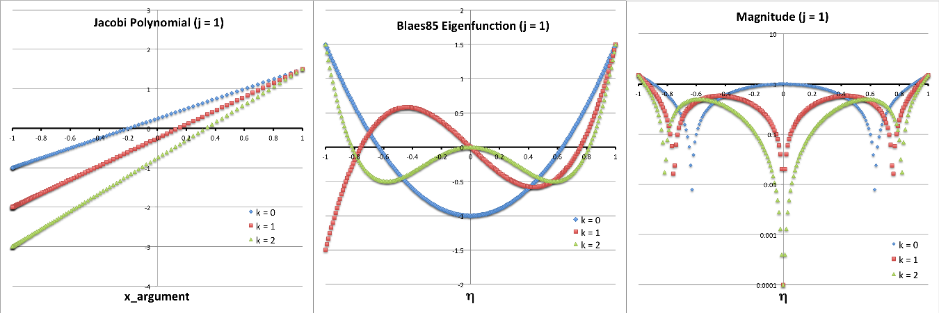
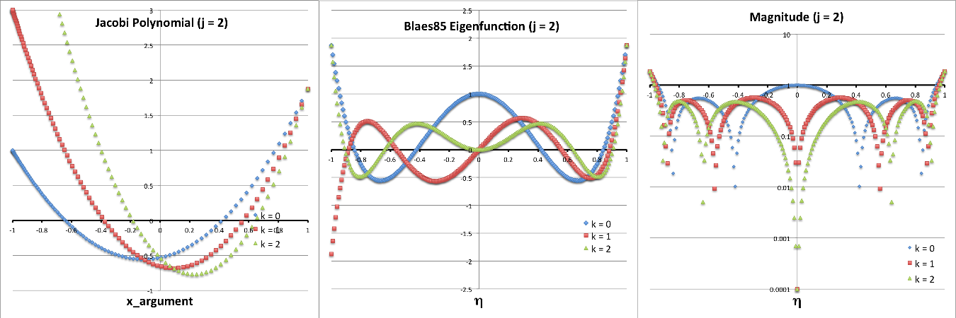
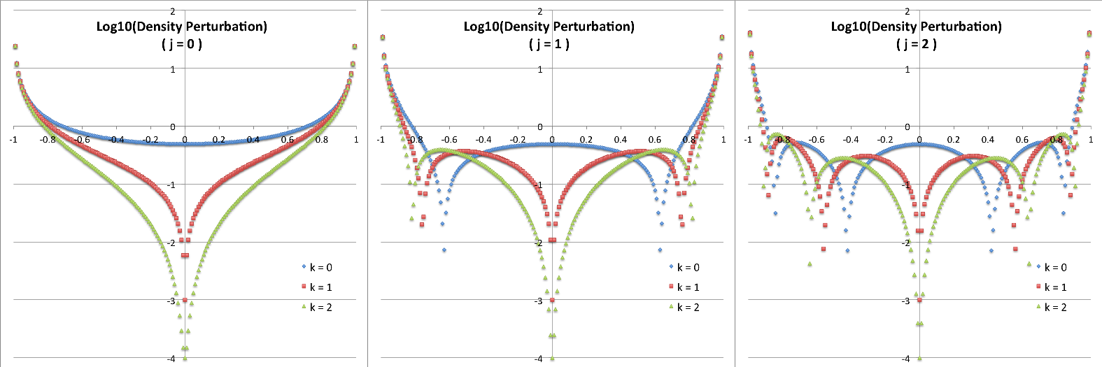
When we began our review of these published studies, we did not expect any of the "slender torus" eigenfunctions catalogued by [http://adsabs.harvard.edu/abs/1985MNRAS.216..553B Blaes (1985)] — other than the "co-rotation mode" having (''j'',''k'') = (0,0) — to be particularly relevant to our review of the unstable modes discussed in Paper I or Paper II of the Imamura & Hadley collaboration because, in the ''massless'' PP tori, all of these modes are stable. However, as is [[#Plots_of_a_Few_Example_Eigenvectors|demonstrated below]], a close association can be drawn between the structure exhibited by an individual radial eigenfunction that develops spontaneously during the numerical simulation of an unstable, self-gravitating tori and the Jacobi-polynomial-based eigenfunction that is defined by a specific (''j'',''k'') quantum-number pair in ''slender'' PP tori. Evidently, certain normal modes of oscillation that exist but are otherwise stable in ''massless'' PP tori become unstable when the self-gravity of the torus/disk is taken into account. Drawing this association in individual torus/disk simulations may help clarify the specific physical mechanism that is responsible for triggering an instability; at the very least, in many cases it should be possible to assign specific quantum-number pairs to — and thereby more precisely catalog — the fastest growing, unstable modes that develop in a wide range of self-gravitating structures. | |||
Now for some details … | |||
==Background== | ==Background== | ||
===Imamura & Hadley Collaboration=== | ===Imamura & Hadley Collaboration=== | ||
Motivated especially by the numerical study of unstable nonaxisymmetric modes provided in [http://adsabs.harvard.edu/abs/2011Ap%26SS.334....1H Paper I] and [http://adsabs.harvard.edu/abs/2014Ap%26SS.353..191H Paper II] of the [[#See_Also|Imamura & Hadley collaboration]], we have embarked on an effort to better understand what sparks the development of a wide range of complex eigenvectors in self-gravitating tori. Of particular interest are "P-", "J-", and "E-modes," such as the ones whose eigenfunctions are illustrated here in Table 1. (Click on a small image in the right-hand column to see a larger image.) Our initial attempts to construct fits to these eigenvectors empirically have been described in [[User:Tohline/Appendix/Ramblings/Azimuthal_Distortions#Analyzing_Azimuthal_Distortions|a separate chapter]]. We begin, here, a more quantitative analysis of these structures. | |||
<table border="1" cellpadding="8" align="center"> | <table border="1" cellpadding="8" align="center"> | ||
<tr> | <tr> | ||
<td align="center" colspan="7"><font size="+1"><b>Table 1:</b></font> P- and E-mode Model Parameters Highlighted in Paper II | <td align="center" colspan="7"><font size="+1"><b>Table 1:</b></font> J-, P- and E-mode Model Parameters Highlighted in Paper II | ||
<p></p>[http://adsabs.harvard.edu/abs/2014Ap%26SS.353..191H K. Z. Hadley, P. Fernandez, J. N. Imamura, E. Keever, R. Tumblin, & W. Dumas (2014, ''Astrophysics and Space Science'', 353, 191-222)]</td> | <p></p>[http://adsabs.harvard.edu/abs/2014Ap%26SS.353..191H K. Z. Hadley, P. Fernandez, J. N. Imamura, E. Keever, R. Tumblin, & W. Dumas (2014, ''Astrophysics and Space Science'', 353, 191-222)]</td> | ||
</tr> | </tr> | ||
<tr> | <tr> | ||
| Line 27: | Line 37: | ||
<td align="center"><math>~R_\mathrm{max}</math></td> | <td align="center"><math>~R_\mathrm{max}</math></td> | ||
<td align="center">Eigenfunction</td> | <td align="center">Eigenfunction</td> | ||
</tr> | |||
<tr> | |||
<td align="center" colspan="6">Extracted from Table 2 of [http://adsabs.harvard.edu/abs/2014Ap%26SS.353..191H Paper II]</td> | |||
<td align="center" colspan="1">Extracted from Fig. 4 of [http://adsabs.harvard.edu/abs/2014Ap%26SS.353..191H Paper II]</td> | |||
</tr> | </tr> | ||
<tr> | <tr> | ||
| Line 54: | Line 68: | ||
<td align="center"><math>~0.159</math></td> | <td align="center"><math>~0.159</math></td> | ||
<td align="center">[[File:ImamuraPaper2Fig4ModelE3.png|175px|Model E3]]</td> | <td align="center">[[File:ImamuraPaper2Fig4ModelE3.png|175px|Model E3]]</td> | ||
</tr> | |||
<tr> | |||
<td align="center" colspan="6">Extracted from Table 2 or Table 4 of [http://adsabs.harvard.edu/abs/2014Ap%26SS.353..191H Paper II]</td> | |||
<td align="center" colspan="1">Extracted from Fig. 3 of [http://adsabs.harvard.edu/abs/2014Ap%26SS.353..191H Paper II]</td> | |||
</tr> | </tr> | ||
<tr> | <tr> | ||
| Line 89: | Line 107: | ||
<td align="center"><math>~1.21</math></td> | <td align="center"><math>~1.21</math></td> | ||
<td align="center"><math>~3.37</math></td> | <td align="center"><math>~3.37</math></td> | ||
<td align="center"> | <td align="center">[[File:ImamuraPaper2Fig3ModelP4.png|175px|Model P4]]</td> | ||
</tr> | |||
<tr> | |||
<td align="center" colspan="6">Extracted from Table 1 of [http://adsabs.harvard.edu/abs/2014Ap%26SS.353..191H Paper II]</td> | |||
<td align="center" colspan="1">Extracted from Fig. 2 of [http://adsabs.harvard.edu/abs/2014Ap%26SS.353..191H Paper II]</td> | |||
</tr> | |||
<tr> | |||
<td align="center">J1</td> | |||
<td align="center"><math>~0.01</math></td> | |||
<td align="center"><math>~(\tfrac{3}{2}, \tfrac{3}{2})</math></td> | |||
<td align="center"><math>~0.402</math></td> | |||
<td align="center"><math>~1.51</math></td> | |||
<td align="center"><math>~6.47</math></td> | |||
<td align="center">[[File:ImamuraPaper2Fig2ModelJ1B.png|175px|Model P4]]</td> | |||
</tr> | </tr> | ||
<tr> | <tr> | ||
| Line 97: | Line 128: | ||
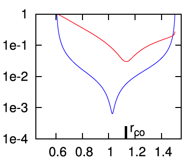
[[File:ImamuraPaper2Fig4Eigenfunction.png|right|250px|Model E2 Radial Eigenfunction]] | [[File:ImamuraPaper2Fig4Eigenfunction.png|right|250px|Model E2 Radial Eigenfunction]]Here, for example, are a couple of questions guiding our study: | ||
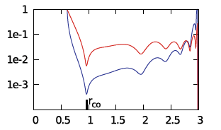
* Can we understand why the radial eigenfunction of, for example, model E2 — re-displayed here, on the right — exhibits a series of sharp dips whose spacing gets progressively smaller and smaller as the outer edge of the torus is approached? | |||
* Does the spatial structure of the unstable eigenvectors that appear in numerical simulations of geometrically thin, self-gravitating tori — such as model "P4" highlighted here in Table 1 — resemble the analytically defined eigenvector that is predicted by linear stability analyses to be unstable in ''massless'' Papaloizou-Pringle tori? | |||
===Radial Modes in Homogeneous Spheres=== | ===Radial Modes in Homogeneous Spheres=== | ||
| Line 359: | Line 392: | ||
<div align="center" id="EigenvaluePP85"> | <div align="center" id="EigenvaluePP85"> | ||
<table border="1" cellpadding="5" width="80%"> | <table border="1" cellpadding="5" width="80%"> | ||
<tr><td align="center"> | <tr><td align="center" bgcolor="orange"> | ||
Equation (2.19) extracted without modification from p. 803 of [http://adsabs.harvard.edu/abs/1985MNRAS.213..799P Papaloizou & Pringle (1985)]<p></p> | Equation (2.19) extracted without modification from p. 803 of [http://adsabs.harvard.edu/abs/1985MNRAS.213..799P Papaloizou & Pringle (1985)]<p></p> | ||
"''The dynamical stability of differentially rotating discs. II''"<p></p> | "''The dynamical stability of differentially rotating discs. II''"<p></p> | ||
| Line 423: | Line 456: | ||
====Setup==== | ====Setup==== | ||
<table border="1" cellpadding="5" align="right"> | <table border="1" cellpadding="5" align="right" width="30%"> | ||
<tr><td align="center"> | <tr><td align="center" bgcolor="orange"> | ||
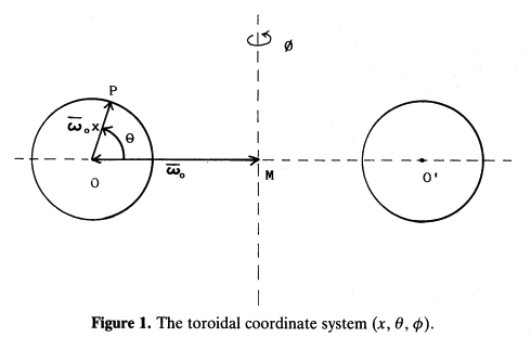
Fig. 1 extracted without modification from p. 554 of [http://adsabs.harvard.edu/abs/1985MNRAS.216..553B Blaes (1985)]<p></p> | Fig. 1 extracted without modification from p. 554 of [http://adsabs.harvard.edu/abs/1985MNRAS.216..553B Blaes (1985)]<p></p> | ||
"''Oscillations of Slender Tori''"<p></p> | "''Oscillations of Slender Tori''"<p></p> | ||
Monthly Notices of the Royal Astronomical Society, < | Monthly Notices of the Royal Astronomical Society, <br />vol. 216, Issue 3, October 1985, pp. 553-563<br />© Royal Astronomical Society<br /> | ||
vol. 216, pp. 553-563 © Royal Astronomical Society | https://doi.org/10.1093/mnras/216.3.553 | ||
</td></tr> | </td></tr> | ||
<tr> | <tr> | ||
<td align="center"> | <td align="center"> | ||
[[File:Blaes85Fig1.png|center|300px|Figure 1 from Blaes (1985)]] | [[File:Blaes85Fig1.png|center|300px|Figure 1 from Blaes (1985)]] | ||
</td> | |||
</tr> | |||
<tr> | |||
<td align="left"> | |||
This digital image has been posted by permission of author, O.M. Blaes (via email dated 19 July 2020), and by permission of Oxford University Press on behalf of the Royal Astronomical Society (via email dated 31 July 2020). | |||
<div align="center">Original publication website: https://academic.oup.com/mnras/article/216/3/553/1005987</div> | |||
</td> | </td> | ||
</tr> | </tr> | ||
| Line 556: | Line 595: | ||
<div align="center" id="EigenvalueBlaes85"> | <div align="center" id="EigenvalueBlaes85"> | ||
<table border="1" cellpadding="5" width="80%"> | <table border="1" cellpadding="5" width="80%"> | ||
<tr><td align="center"> | <tr><td align="center" bgcolor="orange"> | ||
Equation (3.2) extracted without modification from p. 558 of [http://adsabs.harvard.edu/abs/1985MNRAS.216..553B Blaes (1985)]<p></p> | Equation (3.2) extracted without modification from p. 558 of [http://adsabs.harvard.edu/abs/1985MNRAS.216..553B O. M. Blaes (1985)]<p></p> | ||
"''Oscillations of Slender Tori''"<p></p> | "''Oscillations of Slender Tori''"<p></p> | ||
Monthly Notices of the Royal Astronomical Society, vol. 216, pp. 553-563 © Royal Astronomical Society | Monthly Notices of the Royal Astronomical Society, vol. 216, Issue 3, October 1985, pp. 553-563<br />© Royal Astronomical Society<br /> | ||
https://doi.org/10.1093/mnras/216.3.553 | |||
</td></tr> | </td></tr> | ||
<tr> | <tr> | ||
| Line 565: | Line 605: | ||
[[File:Blaes85Eq3.2.png|600px|center|Blaes (1985, MNRAS, 216, 553)]] | [[File:Blaes85Eq3.2.png|600px|center|Blaes (1985, MNRAS, 216, 553)]] | ||
<!-- [[Image:AAAwaiting01.png|400px|center|Whitworth (1981) Eq. 5]] --> | <!-- [[Image:AAAwaiting01.png|400px|center|Whitworth (1981) Eq. 5]] --> | ||
</td> | |||
</tr> | |||
<tr> | |||
<td align="left"> | |||
This digital image has been posted by permission of author, O.M. Blaes (via email dated 19 July 2020), and by permission of Oxford University Press on behalf of the Royal Astronomical Society (via email dated 31 July 2020). | |||
<div align="center">Original publication website: https://academic.oup.com/mnras/article/216/3/553/1005987</div> | |||
</td> | </td> | ||
</tr> | </tr> | ||
| Line 615: | Line 661: | ||
<div align="center" id="EigenvalueBlaes85"> | <div align="center" id="EigenvalueBlaes85"> | ||
<table border="1" cellpadding="5" width="80%"> | <table border="1" cellpadding="5" width="80%"> | ||
<tr><td align="center"> | <tr><td align="center" bgcolor="orange"> | ||
Equation (1.6) — identical to Eq. (3.5) — extracted without modification from p. 555 of [http://adsabs.harvard.edu/abs/1985MNRAS.216..553B Blaes (1985)]<p></p> | Equation (1.6) — identical to Eq. (3.5) — extracted without modification from p. 555 of [http://adsabs.harvard.edu/abs/1985MNRAS.216..553B O. M. Blaes (1985)]<p></p> | ||
"''Oscillations of Slender Tori''"<p></p> | "''Oscillations of Slender Tori''"<p></p> | ||
Monthly Notices of the Royal Astronomical Society, vol. 216, pp. 553-563 © Royal Astronomical Society | Monthly Notices of the Royal Astronomical Society, vol. 216, Issue 3, October 1985, pp. 553-563<br />© Royal Astronomical Society<br /> | ||
https://doi.org/10.1093/mnras/216.3.553 | |||
</td></tr> | </td></tr> | ||
<tr> | <tr> | ||
<td align="center"> | <td align="center"> | ||
[[File:Blaes85Eq1.6.png|600px|center|Blaes (1985, MNRAS, 216, 553)]] | [[File:Blaes85Eq1.6.png|600px|center|Blaes (1985, MNRAS, 216, 553)]] | ||
<!-- [[Image:AAAwaiting01.png|400px|center|Whitworth (1981) Eq. 5]] --> | |||
</td> | |||
</tr> | |||
<tr> | |||
<td align="left"> | |||
This digital image has been posted by permission of author, O.M. Blaes (via email dated 19 July 2020), and by permission of Oxford University Press on behalf of the Royal Astronomical Society (via email dated 31 July 2020). | |||
<div align="center">Original publication website: https://academic.oup.com/mnras/article/216/3/553/1005987</div> | |||
</td> | </td> | ||
</tr> | </tr> | ||
| Line 1,020: | Line 1,074: | ||
</div> | </div> | ||
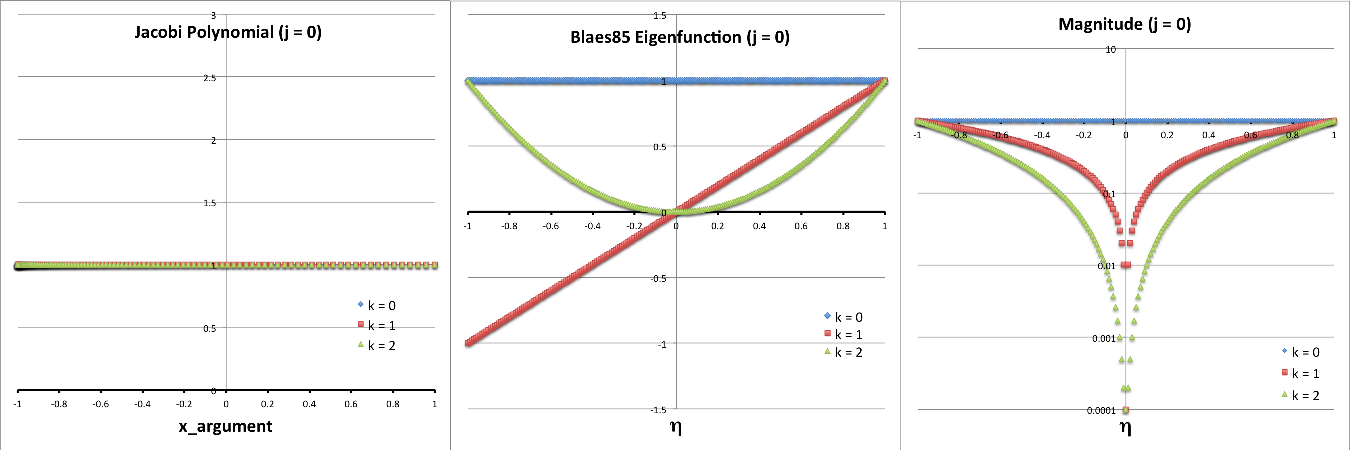
where, <math>~C</math> is an arbitrary, overall scale factor. A plot showing the radial structure of this "simplest mode" — assuming <math>~C=1</math> — is provided by the blue curve in the middle segment and in the right-hand segment of panel A. The perturbation has a constant amplitude throughout the configuration. Note, however, that as the left-most segment of panel D in Figure 2 shows, the fractional ''density'' perturbation is not uniform throughout the configuration; this is primarily because an extra factor of <math>~(1-\eta^2)^{-1}</math> appears in the expression for <math>~\rho^'/\rho_0</math> — [[#DensityPerturbation2|see above]]. | where, <math>~C</math> is an arbitrary, overall scale factor. A plot showing the radial structure of this "simplest mode" — assuming <math>~C=1</math> — is provided by the blue curve in the middle segment and in the right-hand segment of panel A. The perturbation, <math>~\delta W_{0,0,m}^{(0)}</math>, has a constant amplitude throughout the configuration. Note, however, that as the left-most segment of panel D in Figure 2 shows, the fractional ''density'' perturbation is not uniform throughout the configuration; this is primarily because an extra factor of <math>~(1-\eta^2)^{-1}</math> appears in the expression for <math>~\rho^'/\rho_0</math> — [[#DensityPerturbation2|see above]]. | ||
While this <font color="maroon"><b>COROTATION</b></font> mode exhibits a rather boring structure relative to other modes, it plays a key role in the Blaes (1985) publication. As his analysis is expanded to include the examination of oscillations in tori with finite — but still small — equilibrium values of <math>~\beta</math>, he finds that, for all ''m'', both the eigenfunction and the eigenfrequency of the ''j'' = ''k'' = 0 mode exhibit nonzero imaginary components. (More on this, [[#Tori_with_Small_but_Finite_.CE.B2|immediately below]].) | While this <font color="maroon"><b>COROTATION</b></font> mode exhibits a rather boring structure relative to other modes, it plays a key role in the Blaes (1985) publication. As his analysis is expanded to include the examination of oscillations in tori with finite — but still small — equilibrium values of <math>~\beta</math>, he finds that, for all ''m'', both the eigenfunction and the eigenfrequency of the ''j'' = ''k'' = 0 mode exhibit nonzero imaginary components. (More on this, [[#Tori_with_Small_but_Finite_.CE.B2|immediately below]].) | ||
| Line 1,047: | Line 1,095: | ||
</table> | </table> | ||
</div> | </div> | ||
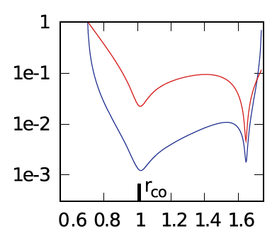
<font color="maroon"><b>MODEL E3 from [http://adsabs.harvard.edu/abs/2014Ap%26SS.353..191H Hadley, et al. (2014)]:</b></font> In the middle segment of Figure 2's panel E, we have re-printed the semi-log plot of the magnitude of the radial eigenfunction that developed in model E3 from [http://adsabs.harvard.edu/abs/2014Ap%26SS.353..191H Hadley, et al. (2014)]. Both curves in the plot exhibit two radial nodes: One associated with the co-rotation radius, which we have purposely aligned with the node at <math>~\eta = 0</math> that appears in the middle segment of panel D; and one that lies between the center of the torus and the surface. This association strongly suggests that the unstable mode found in model E3 displays an underlying ''linear'' radial eigenfunction akin to the "''j'' = 1" Jacobi polynomial. Also, because the model E3 eigenfunction exhibits a node at co-rotation, we conclude that <math>~k \ne 0</math>; and, while the spacing between the two E3 nodes suggests a value of the index ''k'' greater than unity, identifying the precise value of ''k'' may require an examination of the node count above/below the equatorial plane along one or more isobaric surfaces. | |||
<font color="maroon"><b>MODEL E2 from [http://adsabs.harvard.edu/abs/2014Ap%26SS.353..191H Hadley, et al. (2014)]:</b></font> In the right-most segment of Figure 2's panel E, we have re-printed the semi-log plot of the magnitude of the radial eigenfunction that developed in model E2 from [http://adsabs.harvard.edu/abs/2014Ap%26SS.353..191H Hadley, et al. (2014)]. In addition to the radial node aligned with co-rotation, both curves in the plot exhibit (at least) four radial nodes. This strongly suggests that this unstable mode displays an underlying radial eigenfunction that is a polynomial of degree, ''j'' = 4 (or higher). | |||
<font color="maroon"><b>MODEL J1 from [http://adsabs.harvard.edu/abs/2014Ap%26SS.353..191H Hadley, et al. (2014)]:</b></font> In the left-most segment of Figure 2's panel E, we have re-printed the semi-log plot of the magnitude of the radial eigenfunction that developed in model J1 from [http://adsabs.harvard.edu/abs/2014Ap%26SS.353..191H Hadley, et al. (2014)]. In all respects, the blue curve (associated with the nonaxisymmetric structure of the density fluctuation) resembles the red curve displayed in the left-most segment of panel D. Because this <font color="maroon"><b>MODEL J1</b></font> eigenfunction exhibits a single radial node that is closely aligned with the center of the torus strongly suggests that the unstable mode corresponds to an oscillation mode having <math>~j = 0</math>, but <math>~k \ne 0</math>. Given its similarity to the red curve in left-most panel of panel D, we suspect that <math>~k = 1</math>. | |||
====Tori with Small but Finite β==== | ====Tori with Small but Finite β==== | ||
| Line 1,088: | Line 1,145: | ||
</div> | </div> | ||
In an accompanying chapter that we have relegated to our | In an [[User:Tohline/Appendix/Ramblings/PPToriPt2#Stability_Analyses_of_PP_Tori_.28Part_2.29|accompanying chapter]] that we have relegated to our [[User:Tohline/Appendix/Ramblings#Ramblings|Ramblings Appendix]], we demonstrate in detail that this pair of ''complex'' expressions does provide a (leading order) solution to the "thick torus" eigenvalue problem. Notice that if <math>~\beta</math> is set to zero, these two expressions reduce to the (purely real) expressions for the ''j'' = ''k'' = 0, slender torus mode. | ||
===Our Additional Analysis=== | |||
====Generic Formulation==== | |||
At any point in time, the fractional density fluctuation associated with any azimuthal mode, <math>~m</math>, can be represented by the expression, | |||
<div align="center"> | |||
<table border="0" cellpadding="5" align="center"> | |||
<tr> | |||
<td align="right"> | |||
<math>~\biggl[ \frac{\rho^'}{\rho_0} \biggr]_m</math> | |||
</td> | |||
<td align="center"> | |||
<math>~=</math> | |||
</td> | |||
<td align="left"> | |||
<math>~g_m(\eta,\theta)e^{im\varphi} \, .</math> | |||
</td> | |||
</tr> | |||
</table> | |||
</div> | |||
In general, we must assume that the function, <math>~g_m</math>, has both a real and an imaginary component, that is, we should assume that, | |||
<div align="center"> | |||
<table border="0" cellpadding="5" align="center"> | |||
<tr> | |||
<td align="right"> | |||
<math>~g_m(\eta,\theta)</math> | |||
</td> | |||
<td align="center"> | |||
<math>~=</math> | |||
</td> | |||
<td align="left"> | |||
<math>~\mathcal{A}(\eta,\theta) + i\mathcal{B}(\eta,\theta) \, ,</math> | |||
</td> | |||
</tr> | |||
</table> | |||
</div> | |||
in which case the square of the modulus of this function is, | |||
<div align="center"> | |||
<table border="0" cellpadding="5" align="center"> | |||
<tr> | |||
<td align="right"> | |||
<math>~|g_m|^2 \equiv g_m \cdot g^*_m </math> | |||
</td> | |||
<td align="center"> | |||
<math>~=</math> | |||
</td> | |||
<td align="left"> | |||
<math>~\mathcal{A}^2 + \mathcal{B}^2 \, .</math> | |||
</td> | |||
</tr> | |||
</table> | |||
</div> | |||
We can rewrite this complex function in the form, | |||
<div align="center"> | |||
<table border="0" cellpadding="5" align="center"> | |||
<tr> | |||
<td align="right"> | |||
<math>~g_m(\eta,\theta)</math> | |||
</td> | |||
<td align="center"> | |||
<math>~=</math> | |||
</td> | |||
<td align="left"> | |||
<math>~|g_m(\eta,\theta)|e^{i[\alpha(\eta,\theta)]} \, ,</math> | |||
</td> | |||
</tr> | |||
</table> | |||
</div> | |||
if the angle, <math>~\alpha(\eta,\theta)</math> is defined such that, | |||
<div align="center"> | |||
<table border="0" cellpadding="5" align="center"> | |||
<tr> | |||
<td align="right"> | |||
<math>~\cos\alpha = \frac{\mathcal{A}}{\sqrt{\mathcal{A}^2 + \mathcal{B}^2}}</math> | |||
</td> | |||
<td align="center"> | |||
and | |||
</td> | |||
<td align="left"> | |||
<math>~\sin\alpha = \frac{\mathcal{B}}{\sqrt{\mathcal{A}^2 + \mathcal{B}^2}}</math> | |||
</td> | |||
</tr> | |||
<tr> | |||
<td align="right"> | |||
<math>~\Rightarrow ~~~~ \alpha</math> | |||
</td> | |||
<td align="center"> | |||
<math>~\equiv</math> | |||
</td> | |||
<td align="left"> | |||
<math>~\tan^{-1}\biggl(\frac{\mathcal{B}}{\mathcal{A}}\biggr) | |||
= \tan^{-1}\biggl[ \frac{\mathrm{Im}(g_m)}{\mathrm{Re}(g_m)} \biggr] | |||
\, .</math> | |||
</td> | |||
</tr> | |||
</table> | |||
</div> | |||
<span id="DensityEigenfunction">Hence, the spatial structure of the eigenfunction can be rewritten as,</span> | |||
<div align="center"> | |||
<table border="0" cellpadding="5" align="center"> | |||
<tr> | |||
<td align="right"> | |||
<math>~\biggl[ \frac{\rho^'}{\rho_0} \biggr]_m</math> | |||
</td> | |||
<td align="center"> | |||
<math>~=</math> | |||
</td> | |||
<td align="left"> | |||
<math>~|g_m(\eta,\theta)| e^{i[\alpha(\eta,\theta)+m\varphi]} \, .</math> | |||
</td> | |||
</tr> | |||
</table> | |||
</div> | |||
From this representation we can see that, at each spatial location, <math>~(\eta,\theta)</math>, the phase angle(s) at which the fractional perturbation exhibits its maximum amplitude, <math>~|g_m|</math>, is identified by setting the exponent of the exponential to zero. That is, | |||
<div align="center"> | |||
<table border="0" cellpadding="5" align="center"> | |||
<tr> | |||
<td align="right"> | |||
<math>~\varphi = \varphi_\mathrm{max}(\eta,\theta)</math> | |||
</td> | |||
<td align="center"> | |||
<math>~\equiv</math> | |||
</td> | |||
<td align="left"> | |||
<math>~-\frac{1}{m}\biggl[\alpha(\eta,\theta) \biggr] | |||
= -\frac{1}{m}\biggl\{ \tan^{-1}\biggl[ \frac{\mathrm{Im}(g_m)}{\mathrm{Re}(g_m)} \biggr] \biggr\} | |||
\, .</math> | |||
</td> | |||
</tr> | |||
</table> | |||
</div> | |||
An equatorial-plane plot of <math>~\varphi_\mathrm{max}(\eta)</math> should produce the "constant phase locus" referenced, for example, in recent papers from the [[User:Tohline/Appendix/Ramblings/To_Hadley_and_Imamura#Summary_for_Hadley_.26_Imamura|Imamura & Hadley collaboration]]. | |||
<!-- COMMENT OUT | |||
It should be noted that the leading (negative) sign that appears on the right-hand side of this expression for <math>~\phi_\mathrm{max}</math> is rather arbitrary, as is the additional <math>~\pi/2</math> phase shift that appears in that right-hand side expression. Henceforth, for simplicity, we will omit both and use, instead, | |||
<div align="center"> | |||
<table border="0" cellpadding="5" align="center"> | |||
<tr> | |||
<td align="right"> | |||
<math>~m\phi_\mathrm{max}(\varpi)</math> | |||
</td> | |||
<td align="center"> | |||
<math>~\equiv</math> | |||
</td> | |||
<td align="left"> | |||
<math>~\tan^{-1}\biggl[ \frac{\mathrm{Re}(f_m)}{\mathrm{Im}(f_m)} \biggr] | |||
\, ,</math> | |||
</td> | |||
</tr> | |||
</table> | |||
</div> | |||
unless and until the sign and/or a global phase shift is needed to adjust the orientation of a "constant phase locus" plot to facilitate comparison with published figures. | |||
--> | |||
====Density Fluctuations in Tori with Small but Finite β==== | |||
The eigenvector that describes density fluctuations in tori with small but finite <math>~\beta</math> is obtained by combining the [[#DensityPerturbation2|above expression]] for <math>~\rho^'/\rho_0</math> in terms of <math>~\delta W</math>, with the expressions for <math>~\delta W_{0,0,m}</math> and <math>~\sigma_{0,0,m}</math> derived by [http://adsabs.harvard.edu/abs/1985MNRAS.216..553B Blaes (1985)] and [[#Tori_with_Small_but_Finite_.CE.B2|summarized above]]. Keeping in mind that the Blaes85 analysis targeted structures with uniform specific angular momentum, which means that, | |||
<div align="center"> | |||
<table border="0" cellpadding="5" align="center"> | |||
<tr> | |||
<td align="right"> | |||
<math>~\frac{\Omega}{\Omega_0}</math> | |||
</td> | |||
<td align="center"> | |||
<math>~=</math> | |||
</td> | |||
<td align="left"> | |||
<math>~\chi^{-2} | |||
= (1 - x\cos\theta)^{-2} \approx (1 + 2\eta\beta\cos\theta ) \, , | |||
</math> | |||
</td> | |||
</tr> | |||
</table> | |||
</div> | |||
we obtain, | |||
<div align="center"> | |||
<table border="0" cellpadding="5" align="center"> | |||
<tr> | |||
<td align="right"> | |||
<math>~\biggl[\frac{\rho^'}{\rho_0}\biggr]_{0,0,m} </math> | |||
</td> | |||
<td align="center"> | |||
<math>~=</math> | |||
</td> | |||
<td align="left"> | |||
<math>~ | |||
\frac{n}{n+1}\biggl[\biggl(\frac{\sigma }{\Omega_0 }\biggr)_{0,0,m} + m\cdot \frac{\Omega}{\Omega_0}\biggr] \frac{\delta W_{0,0,m}}{f} | |||
</math> | |||
</td> | |||
</tr> | |||
<tr> | |||
<td align="right"> | |||
| |||
</td> | |||
<td align="center"> | |||
<math>~\approx</math> | |||
</td> | |||
<td align="left"> | |||
<math>~ | |||
\frac{C}{(1-\eta^2)}\biggl(\frac{n}{n+1}\biggr)\biggl\{ | |||
\biggl[-m - ~i~m\biggl( \frac{3}{2n+2} \biggr)^{1/2}\beta\biggr] + m (1 + 2\eta\beta\cos\theta ) | |||
\biggr\} e^{[i(m\varphi + \sigma_{0,0,m} t)]} | |||
</math> | |||
</td> | |||
</tr> | |||
<tr> | |||
<td align="right"> | |||
<math>~</math> | |||
</td> | |||
<td align="center"> | |||
<math>~</math> | |||
</td> | |||
<td align="left"> | |||
<math>~ | |||
\times ~ \biggl\{ | |||
1 + \beta^2 m^2\biggl[ | |||
2\eta^2 \cos^2\theta - \frac{3\eta^2}{4(n+1)} - \frac{(4n+1)}{4(n+1)^2} ~\pm ~4i \biggl( \frac{3}{2n+2} \biggr)^{1/2}\eta\cos\theta | |||
\biggr]\biggr\} | |||
</math> | |||
</td> | |||
</tr> | |||
<tr> | |||
<td align="right"> | |||
| |||
</td> | |||
<td align="center"> | |||
<math>~\approx</math> | |||
</td> | |||
<td align="left"> | |||
<math>~ | |||
\frac{C}{(1-\eta^2)}\biggl(\frac{n}{n+1}\biggr)e^{[i(m\varphi + \sigma_{0,0,m} t)]} \biggl[ | |||
\mathrm{Re}(\Delta) + i~\mathrm{Im}(\Delta) | |||
\biggr] \, , | |||
</math> | |||
</td> | |||
</tr> | |||
</table> | |||
</div> | |||
where, | |||
<div align="center"> | |||
<table border="0" cellpadding="5" align="center"> | |||
<tr> | |||
<td align="right"> | |||
<math>~\mathrm{Re}(\Delta)</math> | |||
</td> | |||
<td align="center"> | |||
<math>~\equiv</math> | |||
</td> | |||
<td align="left"> | |||
<math>~ | |||
2\eta(\beta m)\cos\theta\biggl\{ 1 + (\beta m)^2\biggl[ | |||
2\eta^2 \cos^2\theta - \frac{3\eta^2}{4(n+1)} - \frac{(4n+1)}{4(n+1)^2} \biggr] \biggr\} | |||
</math> | |||
</td> | |||
</tr> | |||
<tr> | |||
<td align="right"> | |||
<math>~</math> | |||
</td> | |||
<td align="center"> | |||
<math>~</math> | |||
</td> | |||
<td align="left"> | |||
<math>~\pm | |||
(\beta m)\biggl[\frac{3}{2(n+1)}\biggr]^{1/2} \biggl\{4(\beta m)^2\biggl[\frac{3}{2(n+1)}\biggr]^{1/2} \eta\cos\theta | |||
\biggr\} | |||
</math> | |||
</td> | |||
</tr> | |||
<tr> | |||
<td align="right"> | |||
<math>~</math> | |||
</td> | |||
<td align="center"> | |||
<math>~=</math> | |||
</td> | |||
<td align="left"> | |||
<math>~2\eta(\beta m)\cos\theta \pm \mathcal{O}(\beta^3) \, ;</math> | |||
</td> | |||
</tr> | |||
<tr> | |||
<td align="right"> | |||
<math>~\mathrm{Im}(\Delta)</math> | |||
</td> | |||
<td align="center"> | |||
<math>~\equiv</math> | |||
</td> | |||
<td align="left"> | |||
<math>~ | |||
-~(\beta m) \biggl[\frac{3}{2(n+1)}\biggr]^{1/2}\biggl\{ 1 + (\beta m)^2\biggl[ | |||
2\eta^2 \cos^2\theta - \frac{3\eta^2}{4(n+1)} - \frac{(4n+1)}{4(n+1)^2} \biggr] \biggr\} | |||
</math> | |||
</td> | |||
</tr> | |||
<tr> | |||
<td align="right"> | |||
<math>~</math> | |||
</td> | |||
<td align="center"> | |||
<math>~</math> | |||
</td> | |||
<td align="left"> | |||
<math>~ | |||
\pm~2\eta (\beta m)\cos\theta \biggl\{ 4(\beta m)^2 \biggl[\frac{3}{2(n+1)}\biggr]^{1/2} \eta\cos\theta\biggr\} | |||
</math> | |||
</td> | |||
</tr> | |||
<tr> | |||
<td align="right"> | |||
<math>~</math> | |||
</td> | |||
<td align="center"> | |||
<math>~=</math> | |||
</td> | |||
<td align="left"> | |||
<math>-~(\beta m) \biggl[\frac{3}{2(n+1)}\biggr]^{1/2} \pm \mathcal{O}(\beta^3) \, .</math> | |||
</td> | |||
</tr> | |||
</table> | |||
</div> | |||
Therefore, at any instant in time, this density eigenfunction can be written in the [[#DensityEigenfunction|form discussed above]], namely, | |||
<div align="center"> | |||
<table border="0" cellpadding="5" align="center"> | |||
<tr> | |||
<td align="right"> | |||
<math>~\biggl[ \frac{\rho^'}{\rho_0} \biggr]_{0,0,m}</math> | |||
</td> | |||
<td align="center"> | |||
<math>~=</math> | |||
</td> | |||
<td align="left"> | |||
<math>~|g_{0,0,m}(\eta,\theta)|\exp\{i[\alpha_{0,0,m}(\eta,\theta)+m\varphi]\} \, ,</math> | |||
</td> | |||
</tr> | |||
</table> | |||
</div> | |||
if we set, | |||
<div align="center"> | |||
<table border="0" cellpadding="5" align="center"> | |||
<tr> | |||
<td align="right"> | |||
<math>~|g_{0,0,m}(\eta,\theta)|</math> | |||
</td> | |||
<td align="center"> | |||
<math>~=</math> | |||
</td> | |||
<td align="left"> | |||
<math>~\frac{C}{(1-\eta^2)}\biggl(\frac{n}{n+1}\biggr)|\Delta| \, ,</math> | |||
</td> | |||
</tr> | |||
</table> | |||
</div> | |||
where, | |||
<div align="center"> | |||
<table border="0" cellpadding="5" align="center"> | |||
<tr> | |||
<td align="right"> | |||
<math>~|\Delta|^2</math> | |||
</td> | |||
<td align="center"> | |||
<math>~\approx</math> | |||
</td> | |||
<td align="left"> | |||
<math>~\biggl[ 2\eta(\beta m)\cos\theta\biggr]^2 + \biggl\{ -~(\beta m) \biggl[\frac{3}{2(n+1)}\biggr]^{1/2} \biggr\}^2 </math> | |||
</td> | |||
</tr> | |||
<tr> | |||
<td align="right"> | |||
| |||
</td> | |||
<td align="center"> | |||
<math>~=</math> | |||
</td> | |||
<td align="left"> | |||
<math>~4(\beta m)^2 \biggl[ \eta^2\cos^2\theta + \frac{3}{8(n+1)} \biggr] \, ; | |||
</math> | |||
</td> | |||
</tr> | |||
</table> | |||
</div> | |||
and if we simultaneously set, | |||
<div align="center"> | |||
<table border="0" cellpadding="5" align="center"> | |||
<tr> | |||
<td align="right"> | |||
<math>~\alpha_{0,0,m}(\eta,\theta)</math> | |||
</td> | |||
<td align="center"> | |||
<math>~=</math> | |||
</td> | |||
<td align="left"> | |||
<math>~\tan^{-1}\biggl[ \frac{\mathrm{Im}(\Delta)}{\mathrm{Re}(\Delta)} \biggr] | |||
\approx \tan^{-1}\biggl\{ \frac{-\sqrt{3/[2(n+1)]}}{2\eta\cos\theta} \biggr\} \, . | |||
</math> | |||
</td> | |||
</tr> | |||
</table> | |||
</div> | |||
We note that, in the case of non-self-gravitating PP tori <math>~(\delta \Phi = 0)</math>, the amplitude of the "perturbed enthalpy" as defined by equation (38) of [http://adsabs.harvard.edu/abs/2014Ap%26SS.353..191H Hadley et al. (2014; Paper II)] is, to within a leading scale factor, just <math>~|\Delta|</math>. Specifically, | |||
<div align="center"> | |||
<table border="0" cellpadding="5" align="center"> | |||
<tr> | |||
<td align="right"> | |||
<math>~\mathcal{W}</math> | |||
</td> | |||
<td align="center"> | |||
<math>~=</math> | |||
</td> | |||
<td align="left"> | |||
<math>~\frac{P_0}{\rho_0}\biggl(\frac{n+1}{n}\biggr) |g_{0,0,m}| + \cancelto{0}{\delta\Phi} | |||
= \biggl(\frac{1-\eta^2}{n}\biggr) |g_{0,0,m}| | |||
= \biggl(\frac{C}{n+1}\biggr) |\Delta| \, . | |||
</math> | |||
</td> | |||
</tr> | |||
</table> | |||
</div> | |||
<div align="center" id="Table5"> | |||
<table border="1" align="center" cellpadding="5"> | |||
<tr><th align="center" colspan="8"> | |||
<font size="+1">Table 5: Density Fluctuations in Tori with <math>~n = \tfrac{3}{2}</math> and Small but Finite</font> <math>~\beta</math> | |||
<p></p> | |||
<font size="+1">… Equatorial plane</font> <math>~~\Rightarrow~~~\cos\theta = \pm 1</math> | |||
</th></tr> | |||
<tr> | |||
<td align="center" rowspan="2"><math>~\eta\cos\theta</math> | |||
<td align="center" rowspan="2"><math>~\frac{|\Delta|}{(\beta m)}</math> | |||
<td align="center" rowspan="2"><math>~\frac{|g_{0,0,m}|}{C(\beta m)}</math> | |||
<td align="center" colspan="3"><math>~\alpha_{0,0,m}+\varphi_\mathrm{shift}</math></td> | |||
<td align="center" colspan="2"><font size="+1"><math>~x\cos\theta</math> | |||
<p></p> | |||
(</font>assuming <math>~\beta = 0.12</math><font size="+1">)</font></td> | |||
</tr> | |||
<tr> | |||
<td align="center">Quadrant</td> | |||
<td align="center"><math>~\varphi_\mathrm{shift}=0</math></td> | |||
<td align="center"><math>~\varphi_\mathrm{shift}=\pi</math></td> | |||
<td align="center" rowspan="1">inner<p></p> | |||
<math>~\cos\theta =-1</math> | |||
</td> | |||
<td align="center" rowspan="1">outer<p></p> | |||
<math>~\cos\theta =+1</math> | |||
</td> | |||
</tr> | |||
<tr> | |||
<td align="center"><math>~-1.00</math></td> | |||
<td align="center"><math>~2.145</math></td> | |||
<td align="center"><math>~\infty</math></td> | |||
<td align="center">3<sup>rd</sup></td> | |||
<td align="center">---</td> | |||
<td align="center"><math>~+3.5111</math></td> | |||
<td align="center"><math>~- 0.1088</math></td> | |||
<td align="center"></td> | |||
</tr> | |||
<tr> | |||
<td align="center"><math>~-0.75</math></td> | |||
<td align="center"><math>~1.688</math></td> | |||
<td align="center"><math>~2.315</math></td> | |||
<td align="center">3<sup>rd</sup></td> | |||
<td align="center">---</td> | |||
<td align="center"><math>~+3.6183</math></td> | |||
<td align="center"><math>~- 0.0833</math></td> | |||
<td align="center">---</td> | |||
</tr> | |||
<tr> | |||
<td align="center"><math>~-0.50</math></td> | |||
<td align="center"><math>~1.265</math></td> | |||
<td align="center"><math>~1.012</math></td> | |||
<td align="center">3<sup>rd</sup></td> | |||
<td align="center">---</td> | |||
<td align="center"><math>~+3.8006</math></td> | |||
<td align="center"><math>~- 0.0569</math></td> | |||
<td align="center">---</td> | |||
</tr> | |||
<tr> | |||
<td align="center"><math>~-0.25</math></td> | |||
<td align="center"><math>~0.922</math></td> | |||
<td align="center"><math>~0.5901</math></td> | |||
<td align="center">3<sup>rd</sup></td> | |||
<td align="center">---</td> | |||
<td align="center"><math>~+4.1392</math></td> | |||
<td align="center"><math>~-0.0292</math></td> | |||
<td align="center">---</td> | |||
</tr> | |||
<tr> | |||
<td align="center"><math>~\mp 0.00</math></td> | |||
<td align="center"><math>~0.775</math></td> | |||
<td align="center"><math>~0.4648</math></td> | |||
<td align="center">---</td> | |||
<td align="center"><math>~-\tfrac{\pi}{2}</math></td> | |||
<td align="center"><math>~\tfrac{3\pi}{2}</math></td> | |||
<td align="center"><math>~0.0</math></td> | |||
<td align="center"><math>~0.0</math></td> | |||
</tr> | |||
<tr> | |||
<td align="center"><math>~+0.25</math></td> | |||
<td align="center"><math>~0.922</math></td> | |||
<td align="center"><math>~0.5901</math></td> | |||
<td align="center">4<sup>th</sup></td> | |||
<td align="center"><math>~-0.9976</math></td> | |||
<td align="center">---</td> | |||
<td align="center">---</td> | |||
<td align="center"><math>~0.0310</math></td> | |||
</tr> | |||
<tr> | |||
<td align="center"><math>~+0.50</math></td> | |||
<td align="center"><math>~1.265</math></td> | |||
<td align="center"><math>~1.012</math></td> | |||
<td align="center">4<sup>th</sup></td> | |||
<td align="center"><math>~-0.6591</math></td> | |||
<td align="center">---</td> | |||
<td align="center">---</td> | |||
<td align="center"><math>~0.0643</math></td> | |||
</tr> | |||
<tr> | |||
<td align="center"><math>~+0.75</math></td> | |||
<td align="center"><math>~1.688</math></td> | |||
<td align="center"><math>~2.315</math></td> | |||
<td align="center">4<sup>th</sup></td> | |||
<td align="center"><math>~-0.4767</math></td> | |||
<td align="center">---</td> | |||
<td align="center">---</td> | |||
<td align="center"><math>~0.1007</math></td> | |||
</tr> | |||
<tr> | |||
<td align="center"><math>~+1.00</math></td> | |||
<td align="center"><math>~2.145</math></td> | |||
<td align="center"><math>~\infty</math></td> | |||
<td align="center">4<sup>th</sup></td> | |||
<td align="center"><math>~-0.3695</math></td> | |||
<td align="center">---</td> | |||
<td align="center">---</td> | |||
<td align="center"><math>~0.1416</math></td> | |||
</tr> | |||
</table> | |||
</div> | |||
The second and third columns of [[#Table5|Table 5]] detail how, respectively, <math>~|\Delta|</math> and <math>~|g_{0,0,m}|</math> vary with location, <math>~-1 \le \eta\cos\theta \le +1</math>, in the equatorial plane <math>~(\cos\theta = \pm 1)</math> of a slim, <math>~n=\tfrac{3}{2}</math> PP torus. Table 5 also contains an evaluation of the phase angle, <math>~\alpha_{0,0,m}</math>, across the equatorial plane of the same torus. As indicated, in making this evaluation, care has been taken to place the phase angle in the proper quadrant of the equatorial plane. Specifically — keeping in mind that, according to Blaes' analytic solution, the numerator of the arctangent argument, <math>~\mathrm{Im}(\Delta)</math>, is always negative — the phase angle should land in either the 3<sup>rd</sup> or 4<sup>th</sup> quadrant depending on whether the denominator is, respectively, negative <math>~(\eta\cos\theta < 0)</math> or positive <math>~(\eta\cos\theta > 0)</math>. Because a standard evaluation of the arctangent function returns an angle that lies either in the 1<sup>st</sup> quadrant (positive argument) or the 4<sup>th</sup> quadrant (negative argument), we have added <math>~\varphi_\mathrm{shift} = \pi</math> to the value returned by the arctangent function in order to push the phase angle from the 1<sup>st</sup> to the 3<sup>rd</sup> quadrant wherever the denominator is negative — that is to say, this phase shift has been implemented, throughout the range, <math>-1 \le \eta\cos\theta < 0</math>. | |||
====Comparison with Results from the Imamura & Hadley Collaboration==== | |||
=====Visual Comparison===== | |||
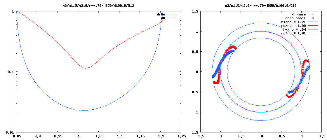
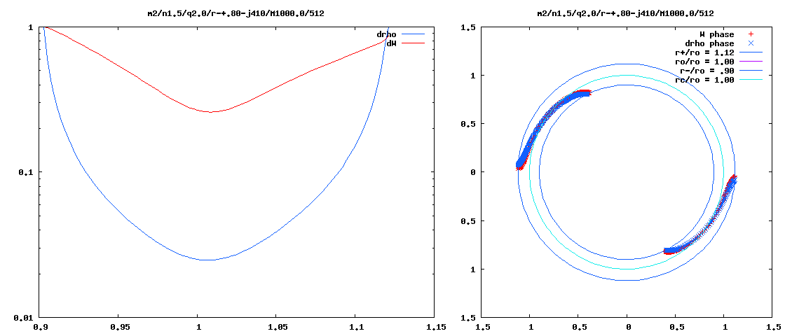
With the above information in hand, we can now directly compare the eigenfunction of the unstable, ''m'' = 2 mode discovered and defined analytically by [http://adsabs.harvard.edu/abs/1985MNRAS.216..553B Blaes (1985)] with the eigenfunction of unstable, ''m'' = 2 modes found by the [[#See_Also|Imamura & Hadley collaboration]] while using numerical hydrodynamic techniques to simulate the evolution of similarly slim tori. Panel A of Figure 3 displays a pair of plots, extracted from [http://adsabs.harvard.edu/abs/2014Ap%26SS.353..191H Hadley et al. (2014; Paper II)], that present information regarding the ''m'' = 2 mode, nonaxisymmetric structure that developed in the equatorial plane of their model P4. The model P4 disk/torus is geometrically slim <math>~(\beta \approx 0.18)</math> and its mass, although not zero, is only 1% of the mass of the central star <math>~(M_*/M_\mathrm{disk} = 10^2)</math>. Panel B of Figure 3 displays a similar pair of plots from a separate, [[User:Tohline/Appendix/Ramblings/Hadley_and_Imamura_Supplementary_Database#Supplementary_Dataset_Generated_by_Hadley_.26_Imamura_Collaboration|unpublished Hadley et al. model evolution]]; in this model, the disk/torus mass is only 0.1% that of the central star <math>~(M_*/M_\mathrm{disk} = 10^3)</math>. In both panels, the blue curves show the geometric structure of non-axisymmetric, equatorial-plane density fluctuations, <math>~|\rho^'/\rho_0|_2</math>, and the red curves show the structure of the "enthalpy + gravity" perturbation, <math>~\mathcal{W}</math>: The left-hand plot displays log<sub>10</sub> of (the modulus of) the amplitude versus radius; while the right-hand plot displays the unstable mode's constant phase locus. In each of these plots, the radial coordinate is, <math>~\chi \equiv \varpi/\varpi_0</math>. | |||
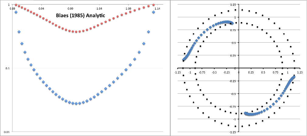
Panel C of Figure 3 presents similar plots that we have generated to show the ''m'' = 2 mode, non-axisymmetric, equatorial-plane density and enthalpy fluctuations predicted by the [http://adsabs.harvard.edu/abs/1985MNRAS.216..553B Blaes (1985)] analysis. More specifically, on the left, we have plotted (blue curve) <math>~\log_{10}|g_{0,0,2}|</math> versus <math>~\chi</math>, for <math>~\beta = 0.12</math> and a normalization coefficient, <math>~C = 4</math>; and (red curve) <math>~\log_{10}\mathcal{W}</math> versus <math>~\chi</math>, where we have used a normalization coefficient, <math>~C = 2</math>. (See the third column of Table 5 for example data values.) On the right, we present an equatorial-plane plot of (see columns five and six of Table 5) the constant phase locus, <math>~\tfrac{1}{2}\alpha_{0,0,2}</math> versus <math>~\chi</math>, and — reflecting the ''m'' = 2 mode structure — its twin phase locus, shifted in entirety by <math>~\pi</math> radians. [Note that, in the right-hand plot we have flipped the sign of <math>~\varphi_\mathrm{max}</math> in order to match the sign convention exhibited by the constant phase locus plots presented by the [[#See_Also|Imamura & Hadley collaboration]].] | |||
<div align="center" id="Figure3"> | |||
<table border="1" align="center" cellpadding="5"> | |||
<tr><th><font size="+1">Figure 3: Comparison</font></th></tr> | |||
<tr><th><font size="+1">Panel A: Model P4 from [http://adsabs.harvard.edu/abs/2014Ap%26SS.353..191H Hadley et al. (2014; Paper II)];</font><p></p> | |||
<math>~M_*/M_\mathrm{disk} = 100</math></th></tr> | |||
<tr><td align="right"> | |||
[[File:Montage01Apart1.png|500px|center|Imamura & Hadley collaboration]] | |||
</td></tr> | |||
<tr><th><font size="+1">Panel B: [[User:Tohline/Appendix/Ramblings/Hadley_and_Imamura_Supplementary_Database#Supplementary_Dataset_Generated_by_Hadley_.26_Imamura_Collaboration|Unpublished model]] from Imamura & Hadley collaboration;</font><p></p> | |||
<math>~M_*/M_\mathrm{disk} = 1000</math></th></tr> | |||
<tr><td align="right"> | |||
[[File:Montage01Apart3.png|500px|center|Imamura & Hadley collaboration]] | |||
</td></tr> | |||
<tr><th><font size="+1">Panel C: [http://adsabs.harvard.edu/abs/1985MNRAS.216..553B Blaes (1985)] Analytic Solution with</font> <math>~(\beta, m, C) = (0.12, 2, 0.25)</math>;<p></p> | |||
<math>~M_*/M_\mathrm{disk} = \infty</math></th></tr> | |||
<tr><td align="right"> | |||
[[File:BlaesAnalyticCombined3.png|500px|center|Analytic Solution from Blaes(1985)]] | |||
</td></tr> | |||
</table> | |||
</div> | |||
=====Details Regarding Radial Coordinate Specification===== | |||
We should emphasize that values of <math>~|\Delta|</math>, <math>~|g_{0,0,2}|</math>, and <math>~\alpha_{0,0,2}</math> that have been tabulated in Table 5 and that have been used to generate the two Panel C plots, were determined from analytic expressions that are functions of the parameter, <math>~\eta</math>, not explicitly functions of the radial coordinate, <math>~\chi</math>. How did we determine <math>~\chi</math> from <math>~\eta</math> ? Noting that, in the equatorial plane, | |||
<div align="center"> | |||
<math>\chi = 1 - x\cos\theta \, ,</math> | |||
</div> | |||
with <math>~\cos\theta = \pm 1</math>, we ''could'' have used the [[#Normal_Modes_in_Slender_Tori|slender torus approximation]], <math>~x \approx \eta\beta</math>, to generate the algebraic mapping, | |||
<div align="center"> | |||
<math>\chi \approx 1 \pm \eta\beta \, .</math> | |||
</div> | |||
This would have produced amplitude curves with reflection symmetry about the torus center <math>~(\chi = 1)</math>, and a "constant phase locus" exhibiting symmetry after double-reflection — reflection about the phase angle, - π/2, as well as about <math>~(\chi = 1)</math>. Instead, here we have adopted [[#Establishing_the_Simpler_Eigenvalue_Problem|the more accurate and more realistic, asymmetric relation]] between <math>~x</math> and <math>~\eta</math>, namely, | |||
<div align="center"> | |||
<math>~x^2 \pm 2x^3 = (\beta\eta)^2 \, .</math> | |||
</div> | |||
In an [[User:Tohline/Appendix/Ramblings/PPTori#Cubic_Equation_Solution|accompanying discussion]], we show that the relevant roots of this cubic equation give, from the inner edge of the torus to the pressure/density maximum, | |||
<div align="center"> | |||
<table border="0" cellpadding="5" align="center"> | |||
<tr> | |||
<td align="right"> | |||
<math>~x_\mathrm{inner}</math> | |||
</td> | |||
<td align="center"> | |||
<math>~\equiv</math> | |||
</td> | |||
<td align="left"> | |||
<math>~\frac{1}{6}\biggl\{1 + 2\cos\biggl[\tfrac{1}{3}\cos^{-1}(1-54\beta^2\eta^2) + \frac{2\pi}{3} \biggr] | |||
\biggr\} \, , | |||
</math> | |||
</td> | |||
</tr> | |||
</table> | |||
</div> | |||
while, from the pressure/density maximum to the outer edge of the torus, | |||
<div align="center"> | |||
<table border="0" cellpadding="5" align="center"> | |||
<tr> | |||
<td align="right"> | |||
<math>~x_\mathrm{outer}</math> | |||
</td> | |||
<td align="center"> | |||
<math>~\equiv</math> | |||
</td> | |||
<td align="left"> | |||
<math>~\frac{1}{6}\biggl\{1 + 2\cos\biggl[\tfrac{1}{3}\cos^{-1}(1-54\beta^2\eta^2) - \frac{2\pi}{3} \biggr] | |||
\biggr\} \, . | |||
</math> | |||
</td> | |||
</tr> | |||
</table> | |||
</div> | |||
Sample values of <math>~x_\mathrm{inner}</math> and <math>~x_\mathrm{outer}</math> are given in the last two columns of Table 5, assuming <math>~\beta = 0.12</math>. In either case, the desired dimensionless radial coordinate is then obtained from the expression, | |||
<div align="center"> | |||
<math>~\chi = 1 + x_\mathrm{inner/outer} \, .</math> | |||
</div> | |||
=====Discussion===== | |||
Figure 3 reveals a remarkably strong resemblance between the eigenfunctions that have been generated using analytic expressions from the [http://adsabs.harvard.edu/abs/1985MNRAS.216..553B Blaes (1985)] analysis, and the curves that have emerged from the [http://adsabs.harvard.edu/abs/2014Ap%26SS.353..191H Hadley et al. (2014)] numerical simulations. There are certainly differences in detail among the corresponding curves. But rather than attributing this to shortcomings in the linear perturbation technique used by Blaes, or errors in the hydrodynamic scheme employed by the Imamura & Hadley collaboration, we suggest that the variations seen are real, and principally due to the effects of self-gravity. When moving from panel C, to panel B, to panel A: | |||
* The red "enthalpy + gravity" curve, <math>~\mathcal{W}(\chi)</math>, maintains its overall shape but the central dip becomes progressively more pronounced. This is presumably because the contribution to this function by the perturbation in the gravitational potential, <math>~\delta\Phi</math>, becomes larger (in an absolute sense) as the star-to-disk mass ratio decreases. | |||
* The blue "density fluctuation" curve becomes very slightly more "rounded." | |||
* The blue "constant phase locus" maintains its overall shape, but its end-to-end length gets progressively shorter. In this regard, the Blaes85 analysis tells us that, for slim ''massless'' PP tori — that is, in the limit of <math>~M_*/M_\mathrm{disk} = \infty</math> — the total angular extent of the "constant phase locus" is <font size="+1">(</font>evaluated, here, for <math>~n = \tfrac{3}{2}</math> and <math>~m=2</math><font size="+1">)</font>, | |||
<div align="center"> | |||
<table border="0" cellpadding="5" align="center"> | |||
<tr> | |||
<td align="right"> | |||
<math>~\Delta \varphi|_\mathrm{tot}</math> | |||
</td> | |||
<td align="center"> | |||
<math>~=</math> | |||
</td> | |||
<td align="left"> | |||
<math>~\frac{1}{m}\biggl\{ \pi - 2\tan^{-1}\biggl[ \frac{3}{8(n+1)} \biggr]^{1/2} \biggr\} = 1.20129~\mathrm{radians} | |||
= 68.83~\mathrm{degrees} \, . | |||
</math> | |||
</td> | |||
</tr> | |||
</table> | |||
</div> | |||
=See Also= | =See Also= | ||
Latest revision as of 20:56, 31 July 2020
Characteristics of Unstable Eigenvectors in Self-Gravitating Tori

|
|---|
| | Tiled Menu | Tables of Content | Banner Video | Tohline Home Page | |
Using numerical hydrodynamic techniques, the Imamura & Hadley collaboration — see especially Paper I and Paper II — has studied the dynamical development of nonaxisymmetric instabilities in toroidal configurations that have a range of "star-to-disk" mass ratios and a wide variety of (initially axisymmetric) geometric structures. Our principal aim, here, is to compare the results of these numerical investigations with what is known, analytically, about normal modes of oscillation and nonaxisymmetric instabilities in massless Papaloizou-Pringle tori. On the analytic side, our focus is on the very informative stability analysis published by Blaes (1985; hereafter, Blaes85).
As we review in detail in an accompanying chapter, and summarize, below, Blaes85 discovered a complete spectrum of oscillation modes for slender tori — catalogued according to the integer quantum numbers, (j,k), in addition to the azimuthal mode numer, m — whose meridional-plane structures and corresponding oscillation frequencies are fully specifiable, analytically. Jacobi polynomials underpin the radial structure of these oscillation modes. Blaes85 showed that all of these "slender torus" oscillation modes have real, rather than imaginary, eigenfrequencies, so all of the modes are dynamically stable.
As Blaes (1985) broadened his analysis to include somewhat thicker PP tori — finite, but still small, values of the order parameter, β — he discovered that the eigenfrequency associated with one — and only one — quantum number pair becomes complex: (j,k) = (0,0). (He found that the associated radial eigenfunction is also complex.) Therefore, for all m, this particular mode is expected to be dynamically unstable. Below, we have compared the equatorial-plane structure of this mode, as specified analytically by the Blaes85 analysis, to the nonaxisymmetric structure associated with unstable P-modes that has developed in simulations of slim tori conducted by the Imamura & Hadley collaboration. The structures are not only qualitatively, but quantitatively very similar. (NOTE: While constructing this comparison, we have come to appreciate for the first time that the imaginary component of the complex radial eigenfunction plays a key role in defining the "constant phase locus" signature of an unstable nonaxisymmetric mode.) This bolsters our confidence in the reliability and applicability of, both, the Blaes85 linear perturbation analysis and the nonlinear simulations presented by the Imamura & Hadley collaboration.
When we began our review of these published studies, we did not expect any of the "slender torus" eigenfunctions catalogued by Blaes (1985) — other than the "co-rotation mode" having (j,k) = (0,0) — to be particularly relevant to our review of the unstable modes discussed in Paper I or Paper II of the Imamura & Hadley collaboration because, in the massless PP tori, all of these modes are stable. However, as is demonstrated below, a close association can be drawn between the structure exhibited by an individual radial eigenfunction that develops spontaneously during the numerical simulation of an unstable, self-gravitating tori and the Jacobi-polynomial-based eigenfunction that is defined by a specific (j,k) quantum-number pair in slender PP tori. Evidently, certain normal modes of oscillation that exist but are otherwise stable in massless PP tori become unstable when the self-gravity of the torus/disk is taken into account. Drawing this association in individual torus/disk simulations may help clarify the specific physical mechanism that is responsible for triggering an instability; at the very least, in many cases it should be possible to assign specific quantum-number pairs to — and thereby more precisely catalog — the fastest growing, unstable modes that develop in a wide range of self-gravitating structures.
Now for some details …
Background
Imamura & Hadley Collaboration
Motivated especially by the numerical study of unstable nonaxisymmetric modes provided in Paper I and Paper II of the Imamura & Hadley collaboration, we have embarked on an effort to better understand what sparks the development of a wide range of complex eigenvectors in self-gravitating tori. Of particular interest are "P-", "J-", and "E-modes," such as the ones whose eigenfunctions are illustrated here in Table 1. (Click on a small image in the right-hand column to see a larger image.) Our initial attempts to construct fits to these eigenvectors empirically have been described in a separate chapter. We begin, here, a more quantitative analysis of these structures.
| Table 1: J-, P- and E-mode Model Parameters Highlighted in Paper II K. Z. Hadley, P. Fernandez, J. N. Imamura, E. Keever, R. Tumblin, & W. Dumas (2014, Astrophysics and Space Science, 353, 191-222) | ||||||
| Name | <math>~M_*/M_d</math> | <math>~(n, q)</math>† | <math>~R_-/R_+</math> | <math>~r_\mathrm{outer} \equiv \frac{R_+}{R_\mathrm{max}}</math> | <math>~R_\mathrm{max}</math> | Eigenfunction |
| Extracted from Table 2 of Paper II | Extracted from Fig. 4 of Paper II | |||||
| E1 | <math>~100</math> | <math>~(\tfrac{3}{2}, 2)</math> | <math>~0.101</math> | <math>~5.52</math> | <math>~0.00613</math> | |
| E2 | <math>~100</math> | <math>~(\tfrac{3}{2}, 2)</math> | <math>~0.202</math> | <math>~2.99</math> | <math>~0.0229</math> | 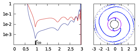 |
| E3 | <math>~100</math> | <math>~(\tfrac{3}{2}, 2)</math> | <math>~0.402</math> | <math>~1.74</math> | <math>~0.159</math> | 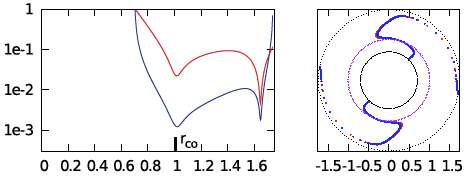 |
| Extracted from Table 2 or Table 4 of Paper II | Extracted from Fig. 3 of Paper II | |||||
| P1 | <math>~100</math> | <math>~(\tfrac{3}{2}, 2)</math> | <math>~0.452</math> | <math>~1.60</math> | <math>~0.254</math> | 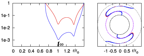 |
| P2 | <math>~100</math> | <math>~(\tfrac{3}{2}, 2)</math> | <math>~0.500</math> | <math>~1.49</math> | <math>~0.403</math> | 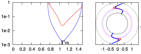 |
| P3 | <math>~100</math> | <math>~(\tfrac{3}{2}, 2)</math> | <math>~0.600</math> | <math>~1.33</math> | <math>~1.09</math> | |
| P4 | <math>~100</math> | <math>~(\tfrac{3}{2}, 2)</math> | <math>~0.700</math> | <math>~1.21</math> | <math>~3.37</math> | 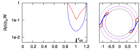 |
| Extracted from Table 1 of Paper II | Extracted from Fig. 2 of Paper II | |||||
| J1 | <math>~0.01</math> | <math>~(\tfrac{3}{2}, \tfrac{3}{2})</math> | <math>~0.402</math> | <math>~1.51</math> | <math>~6.47</math> | 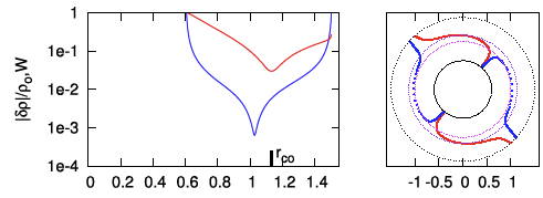 |
| †In all three papers from the Imamura & Hadley collaboration, <math>~q = 2</math> means, "uniform specific angular momentum." | ||||||
Here, for example, are a couple of questions guiding our study:
- Can we understand why the radial eigenfunction of, for example, model E2 — re-displayed here, on the right — exhibits a series of sharp dips whose spacing gets progressively smaller and smaller as the outer edge of the torus is approached?
- Does the spatial structure of the unstable eigenvectors that appear in numerical simulations of geometrically thin, self-gravitating tori — such as model "P4" highlighted here in Table 1 — resemble the analytically defined eigenvector that is predicted by linear stability analyses to be unstable in massless Papaloizou-Pringle tori?
Radial Modes in Homogeneous Spheres
Before attempting to analyze natural modes of oscillation in a polytropic torus, it is useful to review what is known about radial oscillations in the geometrically simpler, uniform-density sphere. As we have reviewed in a separate chapter, Sterne (1937) was the first to recognize that the set of eigenvectors that describe radial modes of oscillation in a homogeneous, self-gravitating sphere can be determined analytically. In the present context, it is advantageous for us to pull Sterne's solution from a discussion of the same problem presented by Rosseland (1964). As we have summarized in a separate chapter, the relevant eigenvalue problem is defined by the following one-dimensional, 2nd-order ODE:
|
<math>~ ( 1-\chi_0^2 ) \frac{\partial^2 \xi}{\partial \chi_0^2} + \frac{2}{\chi_0}\biggl[ 1 - 2\chi_0^2 \biggr] \frac{\partial \xi}{\partial \chi_0} + \biggl(4 - \frac{2}{\chi_0^2} \biggr) \xi</math> |
<math>~=</math> |
<math>~ - \mathfrak{F} \xi \, , </math> |
where, it is understood that the expression for the (spatially and temporally varying) radial location of each spherical shell is,
<math>~r(r_0,t) = r_0 + \delta r(r_0)e^{i\sigma t} \, ,</math>
and in the present context we are adopting the variable notation,
|
<math>~\chi_0</math> |
<math>~\equiv</math> |
<math>~\frac{r_0}{R} \, ,</math> |
|
<math>~\xi</math> |
<math>~\equiv</math> |
<math>~\frac{\delta r}{R} \, ,</math> |
and <math>~R</math> is the initial (unperturbed) radius of the sphere. Here, the eigenvalue is related to the physical properties of the homogeneous sphere via the relation,
<math>~\mathfrak{F} \equiv \frac{2}{\gamma_\mathrm{g}} \biggl[\biggl(\frac{3\sigma^2}{4\pi G\rho_0}\biggr) + (4 - 3\gamma_\mathrm{g}) \biggr] \, .</math>
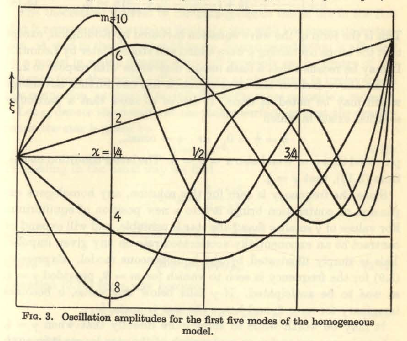
Drawing from Rosseland's (1964) presentation — see his p. 29, and our related discussion — the following table details the eigenvectors (radial eigenfunction and associated eigenfrequency) for the three lowest radial modes (m = 2, 4, 6) that satisfy this wave equation; the figure displayed in the right-most column has been extracted directly from p. 29 of Rosseland and shows the behavior of the lowest five radial modes (m = 2, 4, 6, 8, 10, as labeled) over the interval <math>~0 \le \chi_0 \le 1</math>.
|
Table 2
Rosseland's (1964) Eigenfunctions for Homogeneous Sphere
Figure in the right-most column extracted from p. 29 of Rosseland (1964)
"The Pulsation Theory of Variable Stars" (New York: Dover Publications, Inc.) |
|||
|---|---|---|---|
| Mode | Eigenfunction | Square of Eigenfrequency:<math>~3\sigma^2/(4\pi G\rho)</math> | |
| <math>~m</math> | As Published | <math>~\frac{m}{2}(m+1)\gamma - 4</math> | |
| <math>~2</math> | <math>~\xi = -2\chi_0</math> | <math>~3\gamma - 4</math> | |
| <math>~4</math> | <math>~\xi = -\frac{20}{3}\chi_0 + \frac{28}{3}\chi_0^3</math> | <math>~10\gamma-4</math> | |
| <math>~6</math> | <math>~\xi = -14\chi_0 + \frac{252}{5} \chi_0^3 - \frac{198}{5} \chi_0^5</math> | <math>~21\gamma-4</math> | |
We should point out that, except for the lowest (m = 2) mode, each of the radial eigenfunctions crosses zero at least once at some location(s) that resides between the center <math>~(\chi_0=0)</math> of and the surface <math>~(\chi_0 = 1)</math> of the sphere. More specifically, for each mode, <math>~m</math>, the number of such radial "nodes" is <math>~(m-2)/2</math>. The locations of these nodes is apparent from even a casual inspection of the figure presented in the right-most column of Table 2.
When these radial modes of oscillation are discussed in the astrophysics literature, the conditions that give rise to a dynamical instability are often emphasized. Specifically, each mode becomes unstable when <math>~\sigma^2</math> becomes negative, which translates into a value of <math>~\gamma < \gamma_\mathrm{crit}(m)</math> — see our related discussion of the properties of eigenfunction solutions in the context of Sterne's (1937) analysis of this stability problem. Here we want to emphasize that all of natural modes of oscillation exist even when the configuration is dynamically stable.
Singular Sturm-Liouville Problem
As we have discussed in a separate chapter, there is a class of eigenvalue problems in the mathematical physics literature that is of the "Singular Sturm-Liouville" type. These problems are governed by a one-dimensional, 2nd-order ODE of the form,
|
<math>~ \lambda \Upsilon(x) </math> |
<math>~=</math> |
<math>~-(1-x)^{-\alpha}(1+x)^{-\beta} \cdot \frac{d}{dx} \biggl[ (1-x)^{\alpha+1}(1+x)^{\beta+1} \cdot \frac{d\Upsilon(x)}{dx} \biggr] </math> |
|
|
<math>~=</math> |
<math>~ (x^2-1)\frac{d^2\Upsilon(x)}{dx^2} + [\alpha - \beta + (\alpha+\beta+2)x]\frac{d\Upsilon(x)}{dx} \, , </math> |
where the pair of exponent values, <math>~(\alpha, \beta) </math>, is set by the specific physical problem, while the eigenfunction, <math>~\Upsilon(x)</math>, and associated eigenfrequency, <math>~\lambda</math>, are to be determined. For any choice of the pair of exponents, there is an infinite number <math>~(j = 0 \rightarrow \infty)</math> of analytically known eigenvectors that satisfy this governing ODE; they are referred to as Jacobi Polynomials. Specifically, the jth eigenfunction is,
|
<math>~\Upsilon_j(x) = J_j^{\alpha,\beta}(x)</math> |
<math>~\equiv</math> |
<math>~(1-x)^{-\alpha}(1+x)^{-\beta} \biggl\{ \frac{(-1)^j}{2^j j!} \cdot \frac{d^j}{dx^j}\biggl[ (1-x)^{j+\alpha}(1+x)^{j+\beta} \biggr] \biggr\} \, ;</math> |
and the corresponding jth eigenvalue is,
|
<math>~\lambda_j^{\alpha,\beta}</math> |
<math>~=</math> |
<math>~j(j+\alpha+\beta + 1) \, .</math> |
Table 3 presents the first three eigenfunctions (j = 0, 1, 2), along with each corresponding eigenfrequency; the figure displayed in the right-most column has been extracted directly from §22 (p. 773) of Abramowitz and Stegun's (1964) Handbook of Mathematical Functions (tenth printing, December 1972, with corrections) and shows the behavior of the lowest five Jacobi polynomials (j = 1, 2, 3, 4, 5, as labeled) over the interval <math>~-1 \le x \le +1</math> and for the specific case of <math>~(\alpha,\beta) = (1.5, - 0.5)</math>.
| Table 3: Example Eigenvector Solutions to the Singular Sturm-Liouville Problem | |||
|---|---|---|---|
| <math>~j</math> | <math>~J_j^{\alpha,\beta}(x)</math> | <math>~\lambda_j^{\alpha,\beta}</math> | 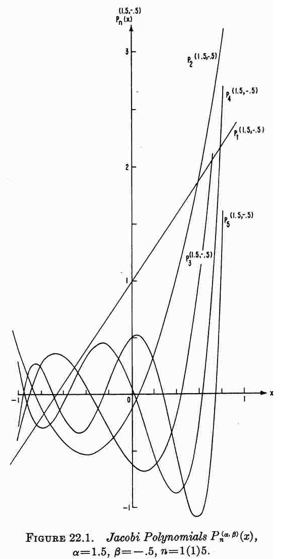 |
|
<math>~0</math> |
<math>~1</math> |
<math>~0</math> |
|
|
<math>~1</math> |
<math>~\tfrac{1}{2}(\alpha+\beta+2)x + \tfrac{1}{2}(\alpha-\beta)</math> |
<math>~(\alpha+\beta+2)</math> |
|
|
<math>~2</math> |
<math>~ \tfrac{1}{8}(12+7\alpha + \alpha^2 + 7\beta+\beta^2+ 2\alpha\beta ) x^2 + \tfrac{1}{4}(3\alpha + \alpha^2 - 3\beta-\beta^2) x + \tfrac{1}{8}(-4 - \alpha + \alpha^2-\beta + \beta^2 - 2\alpha\beta) </math> |
<math>~2(\alpha+\beta+3)</math> |
|
| See also, eqs. (35)-(37) of Wolfram MathWorld; and §22 (p. 773) of Abramowitz and Stegun's (1964) Handbook of Mathematical Functions, from which the illustration on the right has been extracted. | |||
Here we highlight the qualitative similarities between the behavior of the set of Jacobi polynomials [figure extracted from Abramowitz and Stegun (1964) and reprinted here in Table 3] and the set of eigenfunctions that describe normal modes of oscillation in homogeneous, self-gravitating spheres [figure extracted from Rosseland (1964) and reprinted here in Table 2]. As we shall presently see, Jacobi polynomials play an important role in illuminating the structure of normal modes of oscillation in Papaloizou-Pringle tori.
Papaloizou-Pringle Tori
Here we briefly summarize the work (published by several groups in the mid-1980s) that has been done to determine the properties of both stable and unstable, nonaxisymmetric oscillation modes in Papaloizou-Pringle tori. In an accompanying chapter we explain in detail how the two-dimensional, 2nd-order PDE that governs the behavior of these modes was derived by each research group.
Papaloizou & Pringle (1985)
Performing their linear stability analysis in cylindrical coordinates, Papaloizou & Pringle (1985) considered temporal and spatial variations in, for example, the pressure of the form,
<math>~p(\varpi,\varphi,z,t) = p_0(\varpi,z) + p^'(\varpi,z)e^{i(m\varphi + \sigma t)} \, .</math>
Rather than focusing on <math>~p^'</math>, however, they chose to build the governing PDE around an enthalpy-like perturbation defined as,
<math>~W(\varpi,z) = \frac{p^'}{\rho_0\bar\sigma} \, ,</math>
where, <math>~\bar\sigma \equiv (\sigma + m\Omega)</math>, and <math>~\Omega(\varpi)</math> is the fluid's circular orbital frequency in the initially axisymmetric, equilibrium torus. The governing PDE appears as equation (2.19) in Papaloizou & Pringle (1985); for convenience and clarity, that key equation has been extracted from their paper and displayed in the following framed image.
|
Equation (2.19) extracted without modification from p. 803 of Papaloizou & Pringle (1985)
"The dynamical stability of differentially rotating discs. II"
Monthly Notices of the Royal Astronomical Society, vol. 213, pp. 799-820 © Royal Astronomical Society |
Note that, in this equation, <math>~\kappa(\varpi)</math> is the (radially dependent) epicyclic frequency in the torus, and <math>~h^'</math> is the radial derivative of the configuration's specific angular momentum. As has been realized by a number of groups — and as we have demonstrated in our accompanying detailed discussion — this governing PDE simplifies considerably when considering only PP tori that have uniform specific angular momentum because both <math>~\kappa^2</math> and <math>~h^'</math> are zero. Hence, also, <math>~D = \bar\sigma^2</math>. For such systems, the governing PDE is,
|
<math>~\frac{ {\bar\sigma}^2 \rho_0^2 W}{\Gamma p_0 } </math> |
<math>~=</math> |
<math>~ - \frac{1}{\varpi} \frac{\partial}{\partial\varpi} \biggl[ \rho_0 \varpi \cdot \frac{\partial W}{\partial \varpi} \biggr] + \frac{\rho_0 m^2 W }{\varpi^2} - \frac{\partial}{\partial z} \biggl(\rho_0 \frac{\partial W}{\partial z} \biggr) \, . </math> |
Fundamentally, this is the governing PDE that Blaes (1985) used in his examination of the stability of PP tori. But he chose to shift to dimensionless variables and to employ a different meridional-plane coordinate system in his analysis. In an accompanying discussion, we show step-by-step how this expression morphs into the governing PDE that serves as the focus of the Blaes85 analysis. In what follows, we provide a brief summary of this mathematical transformation.
For later use, let's show how the eigenfunction for the density perturbation, <math>~\rho^'</math>, can be obtained from <math>~W</math>. We have,
|
<math>~\rho^'</math> |
<math>~=</math> |
<math>~\frac{\rho_0 p^'}{\gamma_g p_0} = \frac{\rho_0^2 \bar\sigma W}{\gamma_g p_0} \, .</math> |
Blaes (1985)
Setup
|
Fig. 1 extracted without modification from p. 554 of Blaes (1985)
"Oscillations of Slender Tori"
Monthly Notices of the Royal Astronomical Society, |
|
This digital image has been posted by permission of author, O.M. Blaes (via email dated 19 July 2020), and by permission of Oxford University Press on behalf of the Royal Astronomical Society (via email dated 31 July 2020). Original publication website: https://academic.oup.com/mnras/article/216/3/553/1005987
|
As is illustrated in his Figure 1 — which we have reprinted for convenience here, on the right — Blaes (1985) shifted from cylindrical coordinates to a (dimensionless) polar-coordinate <math>~(x,\theta)</math> system whose origin sits at the pressure-maximum of the initial, unperturbed Papaloizou-Pringle torus, a distance, <math>~\varpi_0</math>, from the symmetry axis of the cylindrical coordinate system. Mapping between these two coordinate systems is accomplished via the relations,
|
<math>~x^2 = \biggl(1-\frac{\varpi}{\varpi_0}\biggr)^2 + \biggl(\frac{z}{\varpi_0}\biggr)^2</math> |
and |
<math>~\theta = \tan^{-1}\biggl[\frac{\zeta}{1-\chi}\biggr] \, ;</math> |
| or | ||
|
<math>~\frac{\varpi}{\varpi_0} = 1 - x\cos\theta</math> |
and |
<math>~\frac{z}{\varpi_0} = x\sin\theta \, .</math> |
Furthermore, he set <math>~\Gamma = (n+1)/n</math>, and rewrote the (initial, unperturbed) equilibrium pressure and density distributions in terms of the dimensionless enthalpy distribution in the PP torus, namely,
|
<math>~p_0 </math> |
<math>~=</math> |
<math>~p_\mathrm{max} f^{n+1}\, ,</math> |
|
<math>~\rho_0 </math> |
<math>~=</math> |
<math>~\rho_\mathrm{max} f^{n}\, ,</math> |
where, the two-dimensional dimensionless enthalpy distribution is,
|
<math>~f(x,\theta) </math> |
<math>~\approx</math> |
<math>~1 - \frac{x^2}{\beta^2}\biggl[ 1 + x(3\cos\theta -\cos^3\theta) \biggr] \, ,</math> |
|
<math>~\beta^2</math> |
<math>~\equiv</math> |
<math>~\frac{2n}{\mathfrak{M}_0^2} \, ,</math> |
and <math>~\mathfrak{M}_0</math> is the Mach number of the circular, azimuthal flow at the pressure and density maximum. It is important to appreciate that <math>~\beta</math> is a dimensionless parameter whose value dictates the relative thickness of the equilibrium torus; slim tori have <math>~\beta \ll 1</math>.
Finally, Blaes replaced the perturbation variable, <math>~W</math>, preferred by Papaloizou & Pringle (1985) with an equivalent but dimensionless perturbation variable,
|
<math>~\delta W \equiv \biggl[ \frac{\Omega_0 \rho_\mathrm{max}}{p_\mathrm{max}} \biggr]W </math> |
<math>~\Rightarrow</math> |
<math>~\frac{\rho^'}{\rho_0} = \biggl(\frac{ \bar\sigma }{\gamma_g \Omega_0 } \biggr) \frac{\delta W}{f} = \frac{n}{n+1}\biggl(\frac{\sigma }{\Omega_0 } + m\cdot \frac{\Omega}{\Omega_0}\biggr) \frac{\delta W}{f} \, ,</math> |
where <math>~\Omega_0</math> is the angular frequency at the pressure and density maximum. [Actually, Blaes (1985) calls this dimensionless variable <math>~W</math>, rather than <math>~\delta W</math>, so care must be taken when published equations from these separate studies are compared.] After working carefully through these modifications — again, see our accompanying discussion for details — Blaes arrives at the governing PDE (his equation 3.2) that is highlighted in the following bordered box. Notice that, in this published expression, <math>~\nu \equiv \sigma/\Omega_0</math>, represents the azimuthal-mode eigenfrequency, normalized to the system's orbital frequency at the origin of the Blaes85 coordinate system.
|
Equation (3.2) extracted without modification from p. 558 of O. M. Blaes (1985)
"Oscillations of Slender Tori"
Monthly Notices of the Royal Astronomical Society, vol. 216, Issue 3, October 1985, pp. 553-563 |
|
This digital image has been posted by permission of author, O.M. Blaes (via email dated 19 July 2020), and by permission of Oxford University Press on behalf of the Royal Astronomical Society (via email dated 31 July 2020). Original publication website: https://academic.oup.com/mnras/article/216/3/553/1005987
|
In a direct analogy with Sterne's (1937) analysis of normal modes of oscillation in homogeneous spheres — discussed above — the ultimate objective here is to determine what two-dimensional eigenfunction(s), <math>~\delta W_j(x,\theta)</math>, and corresponding eigenfrequency(ies), <math>~\nu_j</math>, satisfy this governing PDE for arbitrarily thick/thin PP tori. In general, both the eigenfunction and corresponding eigenfrequency should be treated as complex functions/numbers. As we summarize, below, Blaes (1985) derived analytic expressions that provide one approximate solution for tori with small, but finite, values of <math>~\beta</math>. But, first, we will briefly review how he derived an entire spectrum of analytically specifiable normal modes in the limit of "slender tori," that is, tori for which <math>~\beta</math> is effectively zero.
Normal Modes in Slender Tori
Establishing the Simpler Eigenvalue Problem
In what he termed the "slender torus approximation," Blaes (1985) found it advantageous to introduce a function, <math>~\eta</math>, defined in terms of the equilibrium enthalpy distribution, <math>~f</math>, such that,
|
<math>~\eta^2 \equiv 1 - f</math> |
<math>~\approx</math> |
<math>~\frac{x^2}{\beta^2}\biggl[ 1 + x(3\cos\theta -\cos^3\theta) \biggr] \, .</math> |
One nice feature of this parameter is that, for all PP tori, its value varies from zero at the density maximum (also the origin of the Blaes85 polar coordinate system) to unity at the surface of the torus. Also, in the thin torus limit <math>~(\beta \ll 1)</math>,
|
<math>~\eta^2</math> |
<math>~\approx</math> |
<math>~\frac{x^2}{\beta^2} \, ,</math> |
so <math>~\eta</math> can effectively be used as the independent radial coordinate in place of <math>~x</math>. As we demonstrate in detail in an accompanying discussion, in the Blaes85 "slender torus approximation," some of the terms in his equation (3.2) governing PDE dominate over others, facilitating simplification. The result — equation (1.6) in Blaes (1985), also displayed in the following bordered box — is a well-defined eigenvalue problem whose solution(s) provide approximate descriptions of normal mode(s) of oscillation in slender PP tori. Notice that Blaes attaches the superscript, (0), to denote eigenvector solutions to this governing PDE are only approximate solutions valid in the slender torus approximation.
|
Equation (1.6) — identical to Eq. (3.5) — extracted without modification from p. 555 of O. M. Blaes (1985)
"Oscillations of Slender Tori"
Monthly Notices of the Royal Astronomical Society, vol. 216, Issue 3, October 1985, pp. 553-563 |
|
This digital image has been posted by permission of author, O.M. Blaes (via email dated 19 July 2020), and by permission of Oxford University Press on behalf of the Royal Astronomical Society (via email dated 31 July 2020). Original publication website: https://academic.oup.com/mnras/article/216/3/553/1005987
|
Trial Eigenfunction
Following Blaes (1985) — see our accompanying discussion for details — If we assume that the eigenfunction is of the form,
|
<math>~\delta W^{(0)}</math> |
<math>~=</math> |
<math>~\biggl[\eta^{|k|} \exp(ik\theta) \biggr] \Upsilon(\eta) \, ,</math> |
we find that the function, <math>~\Upsilon(\eta)</math>, must satisfy the one-dimensional, 2nd-order ODE,
|
<math>~(1-\eta^2) \frac{d^2\Upsilon}{d\eta^2} + \frac{1}{\eta}\biggl[(2|k|+1) - (2|k|+1+2n)\eta^2\biggr]\frac{d\Upsilon}{d\eta} </math> |
<math>~=</math> |
<math>~ - 2n \biggl[\biggl( \frac{\sigma}{\Omega_0} + m \biggr)^2 -|k|\biggr] \Upsilon \, , </math> |
which is a fairly standard looking eigenvalue problem. If, furthermore, we adopt an independent variable given by the expression,
<math>\Lambda \equiv 2\eta^2 - 1 \, ,</math>
in which case,
<math>\frac{d}{d\eta} \rightarrow 2^{3/2} (\Lambda+1 )^{1/2}\frac{d}{d\Lambda}</math> and <math>\frac{d^2}{d\eta^2} \rightarrow \biggl[ 4\frac{d}{d\Lambda} + 8(\Lambda+1)\frac{d^2}{d\Lambda^2} \biggr] \, , </math>
the statement of the eigenvalue problem becomes,
|
<math>~ \frac{n}{2} \biggl[\biggl( \frac{\sigma}{\Omega_0} + m \biggr)^2 -|k|\biggr] \Upsilon </math> |
<math>~=</math> |
<math>~ (\Lambda^2-1)\frac{d^2\Upsilon}{d\Lambda^2} + \biggl[(n - |k|-1 ) + (|k|+1+n)\Lambda\biggr] \frac{d\Upsilon}{d\Lambda} \, . </math> |
This definition of the eigenvalue problem is exactly of the singular Sturm-Liouville form, as described above, from which we draw the following coefficient associations:
<math>~(\alpha - \beta) \leftrightarrow (n-|k|-1)</math> and <math>~(\alpha+\beta+2) \leftrightarrow (|k|+1+n) \, ,</math>
that is,
<math>~\alpha \leftrightarrow (n-1)</math> and <math>~\beta\leftrightarrow |k|\, .</math>
Hence the jth solution to this eigenvalue problem is,
|
<math>~\Upsilon_j(\Lambda)</math> |
<math>~=</math> |
<math>~J_j^{n-1,|k|}(\Lambda) \, ,</math> |
with the associated eigenvalue,
|
<math>~\frac{n}{2}\biggl[\biggl( \frac{\sigma}{\Omega_0} + m \biggr)_j^2 -|k|\biggr] </math> |
<math>~=</math> |
<math>~j(j+n + |k|)</math> |
|
<math>~\Rightarrow~~~ \biggl( \frac{\sigma}{\Omega_0} + m \biggr)_j^2 </math> |
<math>~=</math> |
<math>~\frac{1}{n}\biggl[2j^2+2jn + 2j|k| + n|k|\biggr] \, .</math> |
Table 4 presents the polynomial expressions that are relevant to the first three (j = 0, 1, 2) eigenfunctions of "slender" PP-tori, along with the associated eigenvalues.
| Table 4: Example Jacobi Polynomials Relevant to "Slender" PP-Tori Eigenvectors | ||
|---|---|---|
| <math>~j</math> | <math>~J_j^{n-1,|k|}(2\eta^2-1)</math> | <math>~\biggl( \frac{\sigma}{\Omega_0} + m \biggr)_j^2</math> |
|
<math>~0</math> |
<math>~1</math> |
<math>~0</math> |
|
<math>~1</math> |
<math>~(n + 1 + |k|)\eta^2 - (1 + |k|)</math> |
<math>~\tfrac{1}{n}[2+2n+(2+n)|k|]</math> |
|
<math>~2</math> |
<math>~ \tfrac{1}{2}[(6 + 5|k|+k^2) +n(5+2|k|) +n^2 ]\eta^4 - [4 + 4|k|+k^2 +n(2+|k|)]\eta^2 + \tfrac{1}{2} [2 + 3|k| + k^2] </math> |
<math>~\tfrac{1}{n}[8+4n + (4+n)|k|] </math> |
Analytic Solution
Piecing this together — including, as well, the time and azimuthal mode, m, dependence — we therefore ultimately conclude that,
|
<math>~\delta W_{j,k,m}^{(0)}</math> |
<math>~=</math> |
<math>~\eta^{|k|} \exp[i(k\theta + m\varphi + \sigma_{j,k,m} t)] ~J_j^{n-1,|k|}(2\eta^2-1) \, ,</math> |
and,
|
<math>~\biggl( \frac{\sigma}{\Omega_0} \biggr)_{j,k,m} </math> |
<math>~=</math> |
<math>~-m \pm \biggl[\frac{2j^2+2jn + 2j|k| + n|k|}{n}\biggr]^{1/2} \, .</math> |
This is a fantastic result, as it provides a totally analytic description of the eigenvectors that define a full spectrum of normal-mode oscillations in slender tori that have uniform specific angular momentum and a range of reasonable polytropic indexes. As Blaes (1985) states — see the discussion immediately following his equation (1.8) — "The three parameters j (a non-negative integer), k (an integer) and m (an integer) completely describe the solution."
Pulling from the expression developed, above, this means that the corresponding density perturbation is,
|
<math>~\biggl(\frac{\rho^'}{\rho_0} \biggr)_{j,k,m}^{(0)}</math> |
<math>~=</math> |
<math>~\frac{n}{n+1}\biggl(\frac{\sigma }{\Omega_0 } + m\biggr)_{j,k,m}^{(0)} \frac{\delta W_{j,k,m}^{(0)}}{f} </math> |
|
|
<math>~=</math> |
<math>~\pm ~\frac{n^{1/2}}{(n+1)} \cdot \frac{\eta^{|k|}}{1-\eta^2}\biggl[2j^2+2jn + 2j|k| + n|k|\biggr]^{1/2} \exp[i(k\theta + m\varphi + \sigma_{j,k,m} t)] ~J_j^{n-1,|k|}(2\eta^2-1) \, . </math> |
We should keep in mind that some restrictions accompany the slender torus approximation.
- Each eigenvector represents a solution of an eigenvalue problem that is simpler than the eigenvalue problem defined by equation (2.19) of Papaloizou & Pringle (1985) — see above — or, equivalently, equation (3.2) of Blaes (1985) — see above.
- In the slender torus, all isobaric surfaces have meridional cross-sections that are perfect circles; and the surface, in particular, has a cross-sectional radius whose value is obtained by setting <math>~\eta = 1 ~~\Rightarrow~~r_\mathrm{torus} = \beta\varpi_0</math>.
And the analytically specified eigenvector exhibits the following simplified attributes:
- As pointed out by Blaes (1985) — see the comments immediately following his equation (1.8) — for all values of <math>~(j,k,m)</math>, the eigenfrequency, <math>~\sigma/\Omega_0</math>, is real, hence all of the identified oscillation modes are stable.
- For all values of <math>~(j,k)</math>, the eigenfunction is real and, as a result, the constant phase locus of each eigenvector will exhibit no azimuthal structure; see more discussion of this attribute, below.
Plots of a Few Example Eigenvectors
Blaes (1985) makes the following brief comments regarding the role of the indices, j and k, in defining the geometric distortions associated with each normal mode. "The significance of k is obvious — it is simply the number of wavelengths on a given isobaric surface [i.e., varying <math>~\theta</math> while holding <math>~\eta</math> constant] so that there are 2k nodal lines radiating from the torus centre at <math>~\eta = 0</math>." Alternatively, moving radially through the torus at a fixed <math>~\theta</math>, "In addition to the [radial] node at <math>~\eta = 0</math> which occurs for <math>~k \ne 0</math>, there are nodal surfaces at j other distinct values of <math>~\eta</math> inside the torus."
The plots presented below in Figures 1 and 2 are intended to further illustrate the radial structure of various normal modes, and to begin to draw a connection between the analytically describable attributes of slender PP tori and the broad range of self-gravitating tori whose stability has been investigated numerically by the Imamura & Hadley collaboration. For nine separate "slender torus" normal modes, panels A, B, & C of Figure 1 display the radial variation of: (Middle) <math>~\delta W_{j,k}^{(0)}</math> versus <math>~\eta</math>; (Left) the associated Jacobi polynomial, <math>~J_{j}^{n-1,|k|}</math> versus <math>~x</math>, where <math>~x = (2\eta^2-1)</math>; and (Right) <math>\log_{10}|\delta W_{j,k}^{(0)}|</math> versus <math>~\eta</math>. In panel A, all three displayed modes have j = 0; in panel B, all modes have j = 1; and in panel C, all modes have j = 2. In all three of these panels (A, B, C), blue curves are associated with k = 0; red curves are associated with k = 1; and green curves are associated with k = 2.
The left-most segment of each panel (A, B, C) displays the specific Jacobi polynomial that seeds the oscillatory behavior of that panel's associated radial eigenvector; they have been shown here in order to emphasize overlap with solutions to the singular Sturm-Liouville problem as illustrated in Table 3, above. In reality, the right-most segment of each panel (A, B, C) presents the same information as is presented in the middle segment, but by plotting the log of the absolute value of the radial eigenfunction we are displaying that information in a manner that aligns with the means of presentation used by the Imamura & Hadley collaboration. Because the log of this function goes to minus infinity whenever the eigenfunction crosses zero, it is particularly easy to identify the number and location of radial nodes in the right-most segment of each panel. Referencing again the comment by Blaes (1985), there is a node at <math>~\eta = 0</math>, except when k = 0 (the blue curves in each panel of our Figure 1); in addition, there are nodal surfaces at j other distinct values of <math>~\eta</math> inside the torus — that is, between <math>~\eta = 0</math> and <math>~\eta = 1</math> or between <math>~\eta = 0</math> and <math>~\eta = -1</math>.
| Figure 1: Blaes85 Eigenfunctions for Slender Tori with <math>~(n,q) = (\tfrac{3}{2},2)</math> |
|---|
| Panel A: j = 0 and (k = 0, 1, 2) |
| Panel B: j = 1 and (k = 0, 1, 2) |
| Panel C: j = 2 and (k = 0, 1, 2) |
COROTATION MODE: As Blaes (1985) has pointed out, for any azimuthal number, m, the simplest mode occurs for j = k = 0. In this case, the analytic expression for the slender torus eigenfrequency is,
|
<math>~\sigma^{(0)}_{0,0,m} </math> |
<math>~=</math> |
<math>~-m \Omega_0 \, ,</math> |
and, the associated analytic expression for the eigenfunction is,
|
<math>~\delta W_{0,0,m}^{(0)}</math> |
<math>~=</math> |
<math>~C ~\exp[i(m\varphi + \sigma^{(0)}_{0,0,m} t)] ~J_0^{n-1,0}(2\eta^2-1) </math> |
|
|
<math>~=</math> |
<math>C~\exp[im(\varphi - \Omega_0 t)] \, ,</math> |
where, <math>~C</math> is an arbitrary, overall scale factor. A plot showing the radial structure of this "simplest mode" — assuming <math>~C=1</math> — is provided by the blue curve in the middle segment and in the right-hand segment of panel A. The perturbation, <math>~\delta W_{0,0,m}^{(0)}</math>, has a constant amplitude throughout the configuration. Note, however, that as the left-most segment of panel D in Figure 2 shows, the fractional density perturbation is not uniform throughout the configuration; this is primarily because an extra factor of <math>~(1-\eta^2)^{-1}</math> appears in the expression for <math>~\rho^'/\rho_0</math> — see above.
While this COROTATION mode exhibits a rather boring structure relative to other modes, it plays a key role in the Blaes (1985) publication. As his analysis is expanded to include the examination of oscillations in tori with finite — but still small — equilibrium values of <math>~\beta</math>, he finds that, for all m, both the eigenfunction and the eigenfrequency of the j = k = 0 mode exhibit nonzero imaginary components. (More on this, immediately below.)
| Figure 2: Mass Density Eigenfunctions for Slender Tori with <math>~(n,q) = (\tfrac{3}{2},2)</math> | ||
|---|---|---|
| Panel D: j = 0 (left), j = 1 (middle), and j = 2 (right) and, in each case, (k = 0, 1, 2) | ||
| Panel E: Models J1 (left), E3 (middle) and E2 (right) from Figs. 2 & 4 of Hadley, et al. (2014) (blue curves show log10 of mass-density fluctuation amplitudes) | ||
MODEL E3 from Hadley, et al. (2014): In the middle segment of Figure 2's panel E, we have re-printed the semi-log plot of the magnitude of the radial eigenfunction that developed in model E3 from Hadley, et al. (2014). Both curves in the plot exhibit two radial nodes: One associated with the co-rotation radius, which we have purposely aligned with the node at <math>~\eta = 0</math> that appears in the middle segment of panel D; and one that lies between the center of the torus and the surface. This association strongly suggests that the unstable mode found in model E3 displays an underlying linear radial eigenfunction akin to the "j = 1" Jacobi polynomial. Also, because the model E3 eigenfunction exhibits a node at co-rotation, we conclude that <math>~k \ne 0</math>; and, while the spacing between the two E3 nodes suggests a value of the index k greater than unity, identifying the precise value of k may require an examination of the node count above/below the equatorial plane along one or more isobaric surfaces.
MODEL E2 from Hadley, et al. (2014): In the right-most segment of Figure 2's panel E, we have re-printed the semi-log plot of the magnitude of the radial eigenfunction that developed in model E2 from Hadley, et al. (2014). In addition to the radial node aligned with co-rotation, both curves in the plot exhibit (at least) four radial nodes. This strongly suggests that this unstable mode displays an underlying radial eigenfunction that is a polynomial of degree, j = 4 (or higher).
MODEL J1 from Hadley, et al. (2014): In the left-most segment of Figure 2's panel E, we have re-printed the semi-log plot of the magnitude of the radial eigenfunction that developed in model J1 from Hadley, et al. (2014). In all respects, the blue curve (associated with the nonaxisymmetric structure of the density fluctuation) resembles the red curve displayed in the left-most segment of panel D. Because this MODEL J1 eigenfunction exhibits a single radial node that is closely aligned with the center of the torus strongly suggests that the unstable mode corresponds to an oscillation mode having <math>~j = 0</math>, but <math>~k \ne 0</math>. Given its similarity to the red curve in left-most panel of panel D, we suspect that <math>~k = 1</math>.
Tori with Small but Finite β
Using perturbation theory with <math>~\beta</math> serving effectively as an order parameter, Blaes (1985) extended his analytic analysis of slender tori to, what he refers to as, "more distorted thick tori." We prefer to describe them as tori with still small, but finite, values of <math>~\beta</math>. Blaes found that, for each m, only the zeroth order co-rotation mode, described above, becomes unstable at higher order. To leading order in <math>~\beta</math>, Blaes shows that (see his equations 1.10 and 1.11) the, now complex, eigenfunction is,
|
<math>~\delta W_{0,0,m}</math> |
<math>~\approx</math> |
<math>~C ~\exp[i(m\varphi + \sigma_{0,0,m} t)] \biggl\{ 1 + \beta^2 m^2\biggl[ 2\eta^2 \cos^2\theta - \frac{3\eta^2}{4(n+1)} - \frac{(4n+1)}{4(n+1)^2} ~\pm ~4i \biggl( \frac{3}{2n+2} \biggr)^{1/2}\eta\cos\theta \biggr]\biggr\} \, , </math> |
and, to leading order in <math>~\beta</math>, the associated complex eigenfrequency is,
|
<math>~\sigma_{0,0,m} </math> |
<math>~\approx</math> |
<math>~-m \Omega_0 - ~i~m\Omega_0 \biggl( \frac{3}{2n+2} \biggr)^{1/2}\beta \, .</math> |
In an accompanying chapter that we have relegated to our Ramblings Appendix, we demonstrate in detail that this pair of complex expressions does provide a (leading order) solution to the "thick torus" eigenvalue problem. Notice that if <math>~\beta</math> is set to zero, these two expressions reduce to the (purely real) expressions for the j = k = 0, slender torus mode.
Our Additional Analysis
Generic Formulation
At any point in time, the fractional density fluctuation associated with any azimuthal mode, <math>~m</math>, can be represented by the expression,
|
<math>~\biggl[ \frac{\rho^'}{\rho_0} \biggr]_m</math> |
<math>~=</math> |
<math>~g_m(\eta,\theta)e^{im\varphi} \, .</math> |
In general, we must assume that the function, <math>~g_m</math>, has both a real and an imaginary component, that is, we should assume that,
|
<math>~g_m(\eta,\theta)</math> |
<math>~=</math> |
<math>~\mathcal{A}(\eta,\theta) + i\mathcal{B}(\eta,\theta) \, ,</math> |
in which case the square of the modulus of this function is,
|
<math>~|g_m|^2 \equiv g_m \cdot g^*_m </math> |
<math>~=</math> |
<math>~\mathcal{A}^2 + \mathcal{B}^2 \, .</math> |
We can rewrite this complex function in the form,
|
<math>~g_m(\eta,\theta)</math> |
<math>~=</math> |
<math>~|g_m(\eta,\theta)|e^{i[\alpha(\eta,\theta)]} \, ,</math> |
if the angle, <math>~\alpha(\eta,\theta)</math> is defined such that,
|
<math>~\cos\alpha = \frac{\mathcal{A}}{\sqrt{\mathcal{A}^2 + \mathcal{B}^2}}</math> |
and |
<math>~\sin\alpha = \frac{\mathcal{B}}{\sqrt{\mathcal{A}^2 + \mathcal{B}^2}}</math> |
|
<math>~\Rightarrow ~~~~ \alpha</math> |
<math>~\equiv</math> |
<math>~\tan^{-1}\biggl(\frac{\mathcal{B}}{\mathcal{A}}\biggr) = \tan^{-1}\biggl[ \frac{\mathrm{Im}(g_m)}{\mathrm{Re}(g_m)} \biggr] \, .</math> |
Hence, the spatial structure of the eigenfunction can be rewritten as,
|
<math>~\biggl[ \frac{\rho^'}{\rho_0} \biggr]_m</math> |
<math>~=</math> |
<math>~|g_m(\eta,\theta)| e^{i[\alpha(\eta,\theta)+m\varphi]} \, .</math> |
From this representation we can see that, at each spatial location, <math>~(\eta,\theta)</math>, the phase angle(s) at which the fractional perturbation exhibits its maximum amplitude, <math>~|g_m|</math>, is identified by setting the exponent of the exponential to zero. That is,
|
<math>~\varphi = \varphi_\mathrm{max}(\eta,\theta)</math> |
<math>~\equiv</math> |
<math>~-\frac{1}{m}\biggl[\alpha(\eta,\theta) \biggr] = -\frac{1}{m}\biggl\{ \tan^{-1}\biggl[ \frac{\mathrm{Im}(g_m)}{\mathrm{Re}(g_m)} \biggr] \biggr\} \, .</math> |
An equatorial-plane plot of <math>~\varphi_\mathrm{max}(\eta)</math> should produce the "constant phase locus" referenced, for example, in recent papers from the Imamura & Hadley collaboration.
Density Fluctuations in Tori with Small but Finite β
The eigenvector that describes density fluctuations in tori with small but finite <math>~\beta</math> is obtained by combining the above expression for <math>~\rho^'/\rho_0</math> in terms of <math>~\delta W</math>, with the expressions for <math>~\delta W_{0,0,m}</math> and <math>~\sigma_{0,0,m}</math> derived by Blaes (1985) and summarized above. Keeping in mind that the Blaes85 analysis targeted structures with uniform specific angular momentum, which means that,
|
<math>~\frac{\Omega}{\Omega_0}</math> |
<math>~=</math> |
<math>~\chi^{-2} = (1 - x\cos\theta)^{-2} \approx (1 + 2\eta\beta\cos\theta ) \, , </math> |
we obtain,
|
<math>~\biggl[\frac{\rho^'}{\rho_0}\biggr]_{0,0,m} </math> |
<math>~=</math> |
<math>~ \frac{n}{n+1}\biggl[\biggl(\frac{\sigma }{\Omega_0 }\biggr)_{0,0,m} + m\cdot \frac{\Omega}{\Omega_0}\biggr] \frac{\delta W_{0,0,m}}{f} </math> |
|
|
<math>~\approx</math> |
<math>~ \frac{C}{(1-\eta^2)}\biggl(\frac{n}{n+1}\biggr)\biggl\{ \biggl[-m - ~i~m\biggl( \frac{3}{2n+2} \biggr)^{1/2}\beta\biggr] + m (1 + 2\eta\beta\cos\theta ) \biggr\} e^{[i(m\varphi + \sigma_{0,0,m} t)]} </math> |
|
<math>~</math> |
<math>~</math> |
<math>~ \times ~ \biggl\{ 1 + \beta^2 m^2\biggl[ 2\eta^2 \cos^2\theta - \frac{3\eta^2}{4(n+1)} - \frac{(4n+1)}{4(n+1)^2} ~\pm ~4i \biggl( \frac{3}{2n+2} \biggr)^{1/2}\eta\cos\theta \biggr]\biggr\} </math> |
|
|
<math>~\approx</math> |
<math>~ \frac{C}{(1-\eta^2)}\biggl(\frac{n}{n+1}\biggr)e^{[i(m\varphi + \sigma_{0,0,m} t)]} \biggl[ \mathrm{Re}(\Delta) + i~\mathrm{Im}(\Delta) \biggr] \, , </math> |
where,
|
<math>~\mathrm{Re}(\Delta)</math> |
<math>~\equiv</math> |
<math>~ 2\eta(\beta m)\cos\theta\biggl\{ 1 + (\beta m)^2\biggl[ 2\eta^2 \cos^2\theta - \frac{3\eta^2}{4(n+1)} - \frac{(4n+1)}{4(n+1)^2} \biggr] \biggr\} </math> |
|
<math>~</math> |
<math>~</math> |
<math>~\pm (\beta m)\biggl[\frac{3}{2(n+1)}\biggr]^{1/2} \biggl\{4(\beta m)^2\biggl[\frac{3}{2(n+1)}\biggr]^{1/2} \eta\cos\theta \biggr\} </math> |
|
<math>~</math> |
<math>~=</math> |
<math>~2\eta(\beta m)\cos\theta \pm \mathcal{O}(\beta^3) \, ;</math> |
|
<math>~\mathrm{Im}(\Delta)</math> |
<math>~\equiv</math> |
<math>~ -~(\beta m) \biggl[\frac{3}{2(n+1)}\biggr]^{1/2}\biggl\{ 1 + (\beta m)^2\biggl[ 2\eta^2 \cos^2\theta - \frac{3\eta^2}{4(n+1)} - \frac{(4n+1)}{4(n+1)^2} \biggr] \biggr\} </math> |
|
<math>~</math> |
<math>~</math> |
<math>~ \pm~2\eta (\beta m)\cos\theta \biggl\{ 4(\beta m)^2 \biggl[\frac{3}{2(n+1)}\biggr]^{1/2} \eta\cos\theta\biggr\} </math> |
|
<math>~</math> |
<math>~=</math> |
<math>-~(\beta m) \biggl[\frac{3}{2(n+1)}\biggr]^{1/2} \pm \mathcal{O}(\beta^3) \, .</math> |
Therefore, at any instant in time, this density eigenfunction can be written in the form discussed above, namely,
|
<math>~\biggl[ \frac{\rho^'}{\rho_0} \biggr]_{0,0,m}</math> |
<math>~=</math> |
<math>~|g_{0,0,m}(\eta,\theta)|\exp\{i[\alpha_{0,0,m}(\eta,\theta)+m\varphi]\} \, ,</math> |
if we set,
|
<math>~|g_{0,0,m}(\eta,\theta)|</math> |
<math>~=</math> |
<math>~\frac{C}{(1-\eta^2)}\biggl(\frac{n}{n+1}\biggr)|\Delta| \, ,</math> |
where,
|
<math>~|\Delta|^2</math> |
<math>~\approx</math> |
<math>~\biggl[ 2\eta(\beta m)\cos\theta\biggr]^2 + \biggl\{ -~(\beta m) \biggl[\frac{3}{2(n+1)}\biggr]^{1/2} \biggr\}^2 </math> |
|
|
<math>~=</math> |
<math>~4(\beta m)^2 \biggl[ \eta^2\cos^2\theta + \frac{3}{8(n+1)} \biggr] \, ; </math> |
and if we simultaneously set,
|
<math>~\alpha_{0,0,m}(\eta,\theta)</math> |
<math>~=</math> |
<math>~\tan^{-1}\biggl[ \frac{\mathrm{Im}(\Delta)}{\mathrm{Re}(\Delta)} \biggr] \approx \tan^{-1}\biggl\{ \frac{-\sqrt{3/[2(n+1)]}}{2\eta\cos\theta} \biggr\} \, . </math> |
We note that, in the case of non-self-gravitating PP tori <math>~(\delta \Phi = 0)</math>, the amplitude of the "perturbed enthalpy" as defined by equation (38) of Hadley et al. (2014; Paper II) is, to within a leading scale factor, just <math>~|\Delta|</math>. Specifically,
|
<math>~\mathcal{W}</math> |
<math>~=</math> |
<math>~\frac{P_0}{\rho_0}\biggl(\frac{n+1}{n}\biggr) |g_{0,0,m}| + \cancelto{0}{\delta\Phi} = \biggl(\frac{1-\eta^2}{n}\biggr) |g_{0,0,m}| = \biggl(\frac{C}{n+1}\biggr) |\Delta| \, . </math> |
|
Table 5: Density Fluctuations in Tori with <math>~n = \tfrac{3}{2}</math> and Small but Finite <math>~\beta</math> … Equatorial plane <math>~~\Rightarrow~~~\cos\theta = \pm 1</math> | |||||||
|---|---|---|---|---|---|---|---|
| <math>~\eta\cos\theta</math> | <math>~\frac{|\Delta|}{(\beta m)}</math> | <math>~\frac{|g_{0,0,m}|}{C(\beta m)}</math> | <math>~\alpha_{0,0,m}+\varphi_\mathrm{shift}</math> | <math>~x\cos\theta</math> (assuming <math>~\beta = 0.12</math>) | |||
| Quadrant | <math>~\varphi_\mathrm{shift}=0</math> | <math>~\varphi_\mathrm{shift}=\pi</math> | inner
<math>~\cos\theta =-1</math> |
outer
<math>~\cos\theta =+1</math> |
|||
| <math>~-1.00</math> | <math>~2.145</math> | <math>~\infty</math> | 3rd | --- | <math>~+3.5111</math> | <math>~- 0.1088</math> | |
| <math>~-0.75</math> | <math>~1.688</math> | <math>~2.315</math> | 3rd | --- | <math>~+3.6183</math> | <math>~- 0.0833</math> | --- |
| <math>~-0.50</math> | <math>~1.265</math> | <math>~1.012</math> | 3rd | --- | <math>~+3.8006</math> | <math>~- 0.0569</math> | --- |
| <math>~-0.25</math> | <math>~0.922</math> | <math>~0.5901</math> | 3rd | --- | <math>~+4.1392</math> | <math>~-0.0292</math> | --- |
| <math>~\mp 0.00</math> | <math>~0.775</math> | <math>~0.4648</math> | --- | <math>~-\tfrac{\pi}{2}</math> | <math>~\tfrac{3\pi}{2}</math> | <math>~0.0</math> | <math>~0.0</math> |
| <math>~+0.25</math> | <math>~0.922</math> | <math>~0.5901</math> | 4th | <math>~-0.9976</math> | --- | --- | <math>~0.0310</math> |
| <math>~+0.50</math> | <math>~1.265</math> | <math>~1.012</math> | 4th | <math>~-0.6591</math> | --- | --- | <math>~0.0643</math> |
| <math>~+0.75</math> | <math>~1.688</math> | <math>~2.315</math> | 4th | <math>~-0.4767</math> | --- | --- | <math>~0.1007</math> |
| <math>~+1.00</math> | <math>~2.145</math> | <math>~\infty</math> | 4th | <math>~-0.3695</math> | --- | --- | <math>~0.1416</math> |
The second and third columns of Table 5 detail how, respectively, <math>~|\Delta|</math> and <math>~|g_{0,0,m}|</math> vary with location, <math>~-1 \le \eta\cos\theta \le +1</math>, in the equatorial plane <math>~(\cos\theta = \pm 1)</math> of a slim, <math>~n=\tfrac{3}{2}</math> PP torus. Table 5 also contains an evaluation of the phase angle, <math>~\alpha_{0,0,m}</math>, across the equatorial plane of the same torus. As indicated, in making this evaluation, care has been taken to place the phase angle in the proper quadrant of the equatorial plane. Specifically — keeping in mind that, according to Blaes' analytic solution, the numerator of the arctangent argument, <math>~\mathrm{Im}(\Delta)</math>, is always negative — the phase angle should land in either the 3rd or 4th quadrant depending on whether the denominator is, respectively, negative <math>~(\eta\cos\theta < 0)</math> or positive <math>~(\eta\cos\theta > 0)</math>. Because a standard evaluation of the arctangent function returns an angle that lies either in the 1st quadrant (positive argument) or the 4th quadrant (negative argument), we have added <math>~\varphi_\mathrm{shift} = \pi</math> to the value returned by the arctangent function in order to push the phase angle from the 1st to the 3rd quadrant wherever the denominator is negative — that is to say, this phase shift has been implemented, throughout the range, <math>-1 \le \eta\cos\theta < 0</math>.
Comparison with Results from the Imamura & Hadley Collaboration
Visual Comparison
With the above information in hand, we can now directly compare the eigenfunction of the unstable, m = 2 mode discovered and defined analytically by Blaes (1985) with the eigenfunction of unstable, m = 2 modes found by the Imamura & Hadley collaboration while using numerical hydrodynamic techniques to simulate the evolution of similarly slim tori. Panel A of Figure 3 displays a pair of plots, extracted from Hadley et al. (2014; Paper II), that present information regarding the m = 2 mode, nonaxisymmetric structure that developed in the equatorial plane of their model P4. The model P4 disk/torus is geometrically slim <math>~(\beta \approx 0.18)</math> and its mass, although not zero, is only 1% of the mass of the central star <math>~(M_*/M_\mathrm{disk} = 10^2)</math>. Panel B of Figure 3 displays a similar pair of plots from a separate, unpublished Hadley et al. model evolution; in this model, the disk/torus mass is only 0.1% that of the central star <math>~(M_*/M_\mathrm{disk} = 10^3)</math>. In both panels, the blue curves show the geometric structure of non-axisymmetric, equatorial-plane density fluctuations, <math>~|\rho^'/\rho_0|_2</math>, and the red curves show the structure of the "enthalpy + gravity" perturbation, <math>~\mathcal{W}</math>: The left-hand plot displays log10 of (the modulus of) the amplitude versus radius; while the right-hand plot displays the unstable mode's constant phase locus. In each of these plots, the radial coordinate is, <math>~\chi \equiv \varpi/\varpi_0</math>.
Panel C of Figure 3 presents similar plots that we have generated to show the m = 2 mode, non-axisymmetric, equatorial-plane density and enthalpy fluctuations predicted by the Blaes (1985) analysis. More specifically, on the left, we have plotted (blue curve) <math>~\log_{10}|g_{0,0,2}|</math> versus <math>~\chi</math>, for <math>~\beta = 0.12</math> and a normalization coefficient, <math>~C = 4</math>; and (red curve) <math>~\log_{10}\mathcal{W}</math> versus <math>~\chi</math>, where we have used a normalization coefficient, <math>~C = 2</math>. (See the third column of Table 5 for example data values.) On the right, we present an equatorial-plane plot of (see columns five and six of Table 5) the constant phase locus, <math>~\tfrac{1}{2}\alpha_{0,0,2}</math> versus <math>~\chi</math>, and — reflecting the m = 2 mode structure — its twin phase locus, shifted in entirety by <math>~\pi</math> radians. [Note that, in the right-hand plot we have flipped the sign of <math>~\varphi_\mathrm{max}</math> in order to match the sign convention exhibited by the constant phase locus plots presented by the Imamura & Hadley collaboration.]
| Figure 3: Comparison |
|---|
| Panel A: Model P4 from Hadley et al. (2014; Paper II); <math>~M_*/M_\mathrm{disk} = 100</math> |
| Panel B: Unpublished model from Imamura & Hadley collaboration; <math>~M_*/M_\mathrm{disk} = 1000</math> |
| Panel C: Blaes (1985) Analytic Solution with <math>~(\beta, m, C) = (0.12, 2, 0.25)</math>; <math>~M_*/M_\mathrm{disk} = \infty</math> |
Details Regarding Radial Coordinate Specification
We should emphasize that values of <math>~|\Delta|</math>, <math>~|g_{0,0,2}|</math>, and <math>~\alpha_{0,0,2}</math> that have been tabulated in Table 5 and that have been used to generate the two Panel C plots, were determined from analytic expressions that are functions of the parameter, <math>~\eta</math>, not explicitly functions of the radial coordinate, <math>~\chi</math>. How did we determine <math>~\chi</math> from <math>~\eta</math> ? Noting that, in the equatorial plane,
<math>\chi = 1 - x\cos\theta \, ,</math>
with <math>~\cos\theta = \pm 1</math>, we could have used the slender torus approximation, <math>~x \approx \eta\beta</math>, to generate the algebraic mapping,
<math>\chi \approx 1 \pm \eta\beta \, .</math>
This would have produced amplitude curves with reflection symmetry about the torus center <math>~(\chi = 1)</math>, and a "constant phase locus" exhibiting symmetry after double-reflection — reflection about the phase angle, - π/2, as well as about <math>~(\chi = 1)</math>. Instead, here we have adopted the more accurate and more realistic, asymmetric relation between <math>~x</math> and <math>~\eta</math>, namely,
<math>~x^2 \pm 2x^3 = (\beta\eta)^2 \, .</math>
In an accompanying discussion, we show that the relevant roots of this cubic equation give, from the inner edge of the torus to the pressure/density maximum,
|
<math>~x_\mathrm{inner}</math> |
<math>~\equiv</math> |
<math>~\frac{1}{6}\biggl\{1 + 2\cos\biggl[\tfrac{1}{3}\cos^{-1}(1-54\beta^2\eta^2) + \frac{2\pi}{3} \biggr] \biggr\} \, , </math> |
while, from the pressure/density maximum to the outer edge of the torus,
|
<math>~x_\mathrm{outer}</math> |
<math>~\equiv</math> |
<math>~\frac{1}{6}\biggl\{1 + 2\cos\biggl[\tfrac{1}{3}\cos^{-1}(1-54\beta^2\eta^2) - \frac{2\pi}{3} \biggr] \biggr\} \, . </math> |
Sample values of <math>~x_\mathrm{inner}</math> and <math>~x_\mathrm{outer}</math> are given in the last two columns of Table 5, assuming <math>~\beta = 0.12</math>. In either case, the desired dimensionless radial coordinate is then obtained from the expression,
<math>~\chi = 1 + x_\mathrm{inner/outer} \, .</math>
Discussion
Figure 3 reveals a remarkably strong resemblance between the eigenfunctions that have been generated using analytic expressions from the Blaes (1985) analysis, and the curves that have emerged from the Hadley et al. (2014) numerical simulations. There are certainly differences in detail among the corresponding curves. But rather than attributing this to shortcomings in the linear perturbation technique used by Blaes, or errors in the hydrodynamic scheme employed by the Imamura & Hadley collaboration, we suggest that the variations seen are real, and principally due to the effects of self-gravity. When moving from panel C, to panel B, to panel A:
- The red "enthalpy + gravity" curve, <math>~\mathcal{W}(\chi)</math>, maintains its overall shape but the central dip becomes progressively more pronounced. This is presumably because the contribution to this function by the perturbation in the gravitational potential, <math>~\delta\Phi</math>, becomes larger (in an absolute sense) as the star-to-disk mass ratio decreases.
- The blue "density fluctuation" curve becomes very slightly more "rounded."
- The blue "constant phase locus" maintains its overall shape, but its end-to-end length gets progressively shorter. In this regard, the Blaes85 analysis tells us that, for slim massless PP tori — that is, in the limit of <math>~M_*/M_\mathrm{disk} = \infty</math> — the total angular extent of the "constant phase locus" is (evaluated, here, for <math>~n = \tfrac{3}{2}</math> and <math>~m=2</math>),
|
<math>~\Delta \varphi|_\mathrm{tot}</math> |
<math>~=</math> |
<math>~\frac{1}{m}\biggl\{ \pi - 2\tan^{-1}\biggl[ \frac{3}{8(n+1)} \biggr]^{1/2} \biggr\} = 1.20129~\mathrm{radians} = 68.83~\mathrm{degrees} \, . </math> |
See Also
- Imamura & Hadley collaboration:
- Paper I: K. Hadley & J. N. Imamura (2011, Astrophysics and Space Science, 334, 1-26), "Nonaxisymmetric instabilities in self-gravitating disks. I. Toroids" — In this paper, Hadley & Imamura perform linear stability analyses on fully self-gravitating toroids; that is, there is no central point-like stellar object and, hence, <math>~M_*/M_d = 0.0</math>.
- Paper II: K. Z. Hadley, P. Fernandez, J. N. Imamura, E. Keever, R. Tumblin, & W. Dumas (2014, Astrophysics and Space Science, 353, 191-222), "Nonaxisymmetric instabilities in self-gravitating disks. II. Linear and quasi-linear analyses" — In this paper, the Imamura & Hadley collaboration performs "an extensive study of nonaxisymmetric global instabilities in thick, self-gravitating star-disk systems creating a large catalog of star/disk systems … for star masses of <math>~0.0 \le M_*/M_d \le 10^3</math> and inner to outer edge aspect ratios of <math>~0.1 < r_-/r_+ < 0.75</math>."
- Paper III: K. Z. Hadley, W. Dumas, J. N. Imamura, E. Keever, & R. Tumblin (2015, Astrophysics and Space Science, 359, article id. 10, 23 pp.), "Nonaxisymmetric instabilities in self-gravitating disks. III. Angular momentum transport" — In this paper, the Imamura & Hadley collaboration carries out nonlinear simulations of nonaxisymmetric instabilities found in self-gravitating star/disk systems and compares these results with the linear and quasi-linear modeling results presented in Papers I and II.

|
|---|
|
© 2014 - 2021 by Joel E. Tohline |
