User:Tohline/ThreeDimensionalConfigurations/ChallengesPt2

Challenges Constructing Ellipsoidal-Like Configurations (Pt. 2)

This chapter extends an accompanying chapter titled, Construction Challenges (Pt. 1). The focus here is on an SCF technique that will incorporate specification of a Lagrangian flow-flied.

Motivation

Example Equilibrium Model

These key parameters have been drawn from [EFE] Chapter 7, Table XIII (p. 170):

<math>~a = a_1 = 1</math>

<math>~b = a_2 = 1.25</math>

<math>~c = a_3 = 0.4703</math>

<math>~\Omega_2 = 0.3639</math>

<math>~\Omega_3 = 0.6633</math>

<math>~\zeta_2 = - 2.2794</math>

<math>~\zeta_3 = - 1.9637</math>

As a consequence — see an accompanying discussion for details — the values of other parameters are …

<math>~\tan\theta </math>	<math>~=</math>	<math>~- \frac{\zeta_2 }{ \zeta_3 } \biggl[ \frac{a^2 + b^2}{a^2 + c^2} \biggr]\frac{c^2}{b^2}</math>	<math>~=</math>	<math>~- 0.00</math>
<math>~ \biggl\{ \biggl[ \frac{a^2}{a^2 + b^2} \biggr] \zeta_3 \cos\theta - \biggl[ \frac{a^2}{a^2 + c^2} \biggr] \zeta_2 \sin\theta \biggr\}y_0 </math>	<math>~=</math>	<math> \biggl[ \frac{a^2}{a^2 + c^2} \biggr] \zeta_2 z_0 </math>	<math>~=</math>	<math>~- 0.00</math>
<math>~ \biggl[ \frac{x_\mathrm{max}}{ y_\mathrm{max} } \biggr]^2 </math>	<math>~=</math>	<math>~ \biggl\{ \biggl[ \frac{a^2}{a^2 + b^2} \biggr] \zeta_3 \cos\theta - \biggl[ \frac{a^2}{a^2 + c^2} \biggr] \zeta_2 \sin\theta \biggr\}\biggl[ \frac{a^2 + b^2}{b^2} \biggr] \frac{\cos\theta}{\zeta_3} </math>	<math>~=</math>	<math>~- 0.00</math>
<math>~ \varphi^2 </math>	<math>~=</math>	<math>~ \biggl\{ \biggl[ \frac{a^2}{a^2 + b^2} \biggr] \zeta_3 - \biggl[ \frac{a^2}{a^2 + c^2} \biggr] \zeta_2 \tan\theta \biggr\}\biggl[ \frac{b^2}{a^2 + b^2} \biggr] \zeta_3 </math>	<math>~=</math>	<math>~- 0.00</math>

COLLADA-Based Representation

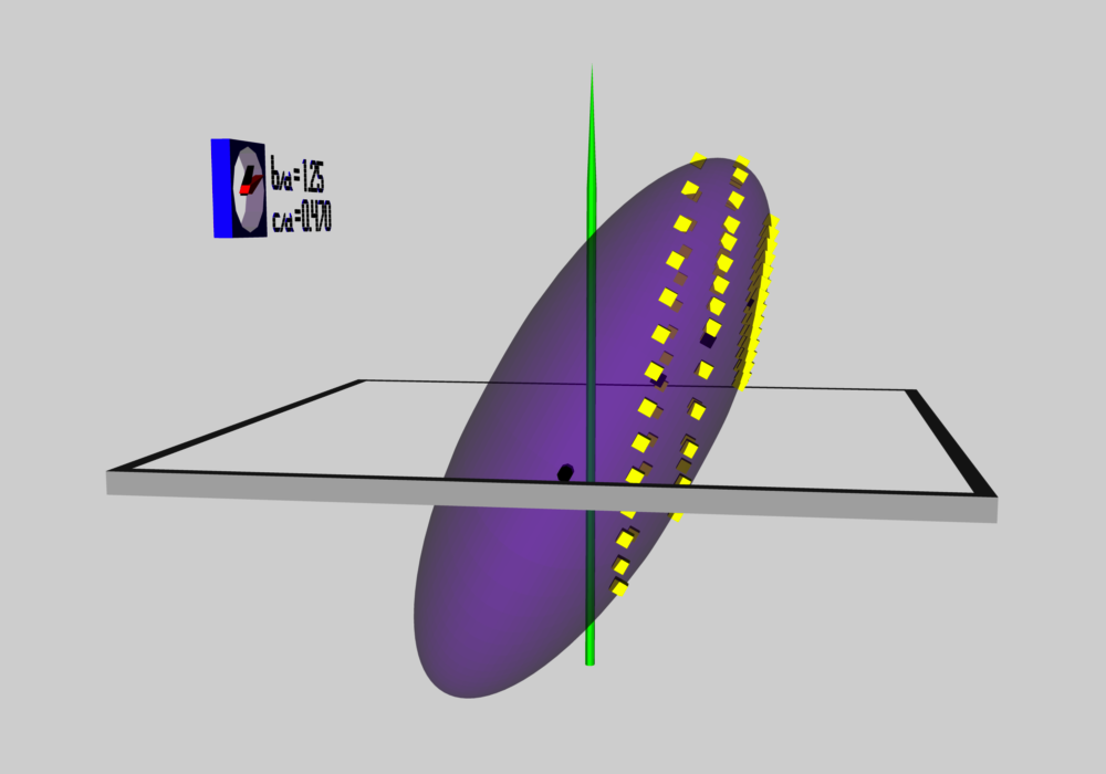
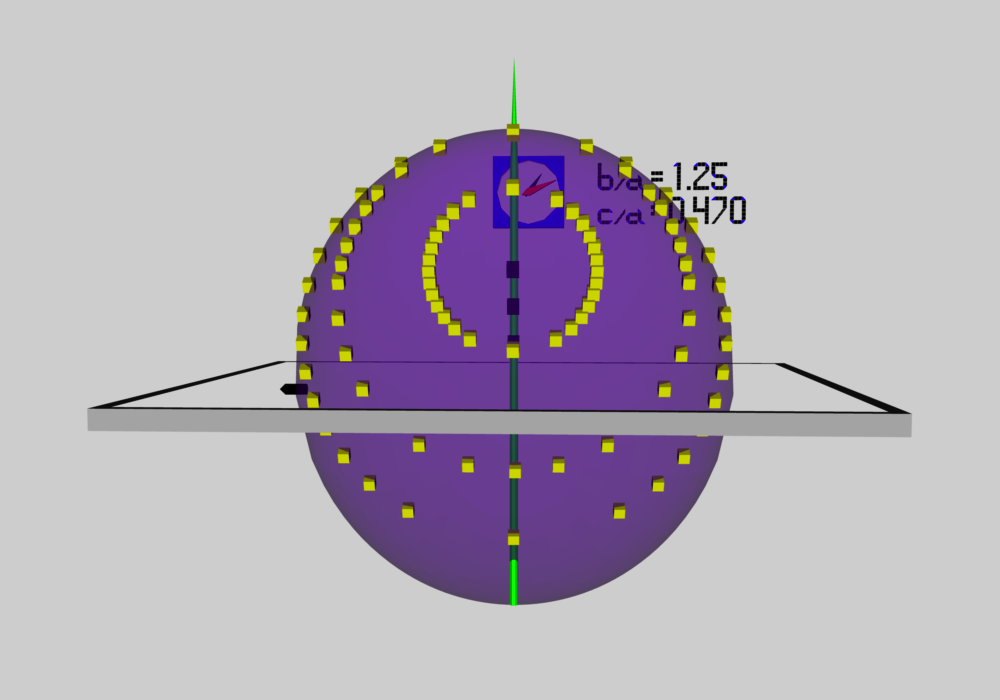
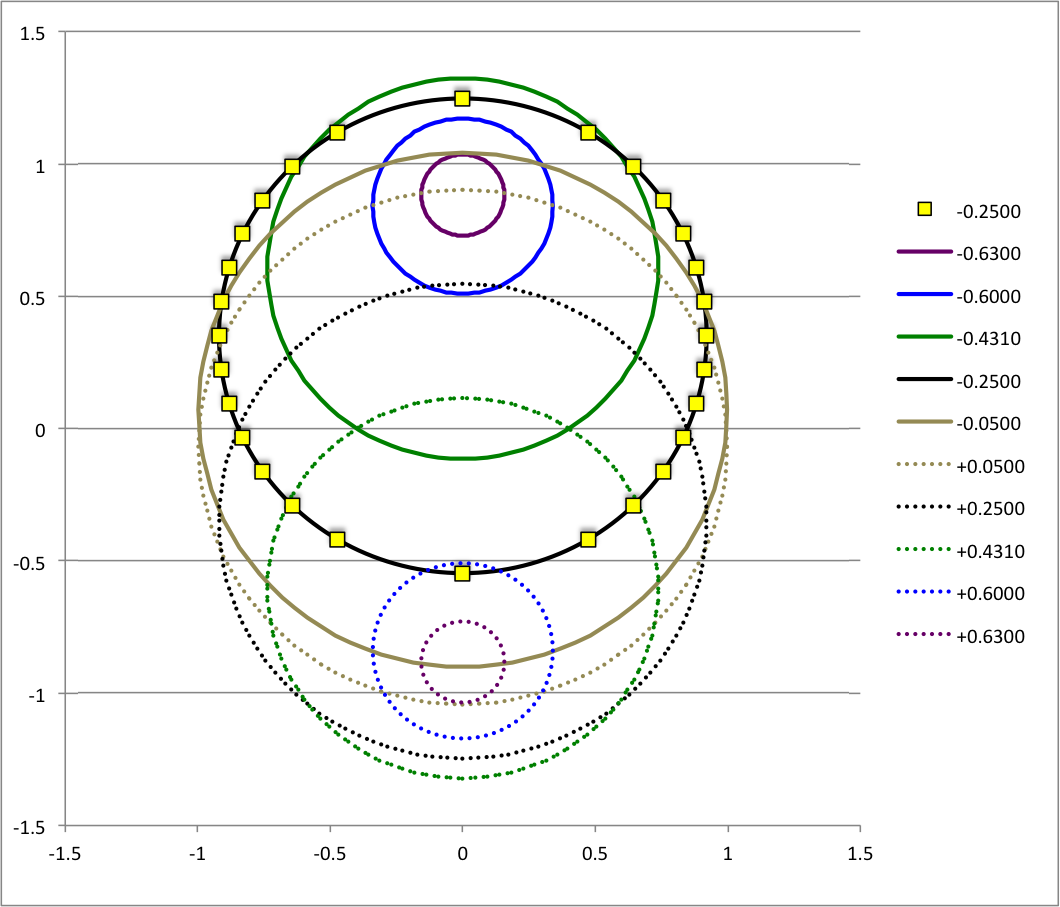
As has been described in an accompanying discussion of Riemann Type 1 ellipsoids, we have used COLLADA to construct an animated and interactive 3D scene that displays in purple the surface of an example Type I ellipsoid; panels a and b of Figure 1 show what this ellipsoid looks like when viewed from two different perspectives. (As a reminder — see the explanation accompanying Figure 2 of that accompanying discussion — the ellipsoid is tilted about the x-coordinate axis at an angle of 61.25° to the equilibrium spin axis, which is shown in green.) Yellow markers also have been placed in this 3D scene at each of the coordinate locations specified in the table that accompanies that discussion. From the perspective presented in Figure 3b, we can immediately identify three separate, nearly circular trajectories; the largest one corresponds to our choice of z₀ = -0.25, the smallest corresponds to our choice of z₀ = -0.60, and the one of intermediate size correspond to our choice of z₀ = -0.4310. When viewed from the perspective presented in Figure 1a, we see that these three trajectories define three separate planes; each plane is tipped at an angle of θ = -19.02° to the untilted equatorial, x-y plane of the purple ellipsoid.

Figure 1a	Figure 1b
↲
Figure 1c
↲

See Also

• Construction Challenges (Pt. 1)
• Riemann Type 1 Ellipsoids

© 2014 - 2021 by Joel E. Tohline |   H_Book Home   |   YouTube   | Appendices: | Equations | Variables | References | Ramblings | Images | myphys.lsu | ADS | Recommended citation:   Tohline, Joel E. (2021), The Structure, Stability, & Dynamics of Self-Gravitating Fluids, a (MediaWiki-based) Vistrails.org publication, https://www.vistrails.org/index.php/User:Tohline/citation