Revision as of 18:56, 9 October 2019

Virtual Reality and 3D Printing

[Circa August 2019] I am once again considering whether steady improvements in certain digital technologies over the past half-a-dozen years can be straightforwardly called upon to display to a broad audience the three-dimensional characteristics of rapidly rotating fluid systems. Two specific technologies come to mind: (1) 3D printing; and (2) XR (virtual reality). A cursory online investigation suggests that we may be able to import OBJ-formatted files into the software algorithms that drive these two technologies. In addition, the popular Unity design tool may serve us well in our efforts to build/view/export such files.

Initial Browsing of Online Resources

DAE files & XML COLLADA format <-- the Preview application on my MacBook Air will open/display a .DAE file

A file with the DAE file extension is a Digital Asset Exchange file. DAE files are based on the COLLADA (COLLAborative Design Activity) XML schema, which is now owned and developed by Autodesk (e.g., Maya). DAE files allow users to transmit 3D graphics files across multiple graphics applications.
Examples:
cube.dae <-- NOTE: I have copied this "dae" file into a dropbox folder and have successfully modified it (changed color from red to purple) inside my txt editor.
In March 2011, Khronos released the COLLADA Conformance Test Suite (CTS). The suite allows applications that import and export COLLADA to test against a large suite of examples, ensuring that they conform properly to the specification. In July 2012, the CTS software was released on GitHub — also see, an associated PDF document, and OpenCOLLADA hosted on Github — allowing for community contributions.
Check out turbosquid.com; or Free3d
August 2013: Autodesk has released Maya LT with COLLADA export capabilities.

Four most common 3D printer file formats in 2019.

STL:
File Format Simply Explained.
As of today, STL is the undisputed champion among 3D printer file formats. STL’s history goes back to the invention of 3D printing itself. The first 3D printer was invented by Chuck Hull in 1987 at 3D Systems. The same guy was behind the STL file format. If you are primarily printing with a single material and in a single color, STL will do the job. But the moment you move to multicolor printing, you have to ditch STL because it is simply not capable of storing colors.
There are many repositories, marketplaces and search engines on the web containing literally millions of free STL files. Thingiverse is probably the largest STL file repository on the internet – so check it out. You can also refer to our regularly updated list: Best Sites for Free STL Files & 3D Printer Models.
STL File Viewers
OBJ:
File format explained.
Format developed by Wavefront; note that a number of the above-referenced STL viewers will also view OBJ files.
AMF
3MF

Try this online 3D converter; in principle, it can be used to convert a DAE (i.e., COLLADA) file to an STL or OBJ file, and visa versa.
Unity

See especially the Products page which briefly refers to …

Platforms: Build once, deploy anywhere to reach the largest possible audience on our industry-leading platform; 25+ platforms across mobile, desktop, console, TV, VR (virtual reality), AR (augmented reality) and the Web.
XR: Powering over two-thirds of VR and AR experiences; Unity is the preferred development tool for the majority of XR creators.

Unreal Engine 4 — competitor of Unity
Oculus Rift S driven by PC; or Oculus Quest, standalone 6DOF VR — looks like they both can be driven by either Unity or Unreal, or via the Native Platform provided by Oculus.

In principle, the Oculus Rift can import new, user-supplied 3D scenes — see the advanced help document — but, for now, it only accepts files in GLB format.
But see the import feature of Oculus Medium 2.0.
GLB format: a binary form of glTF that includes textures instead of referencing them as external images.
glTF: (derivative short form of GL Transmission Format) is a file format for 3D scenes and models using the JSON standard. It is an API-neutral runtime asset delivery format developed by the Khronos Group 3D Formats Working Group. It was announced at HTML5DevConf 2016. This format is intended to be an efficient, interoperable format with minimum file size and runtime processing by apps. As such, its creators have described it as the "JPEG of 3D."

Gear VR — Samsung's headset (powered by Oculus)
GearVR Framework is the SDK for Samsung's Gear VR.
Also consider Oculus Go
vtk has vtkOBJExporter as well as vtkOBJReader
Kitware may also be relevant
Jinghua Ge's CCT-based visualization lab course
Look into the VR Model Viewer from MindRend Technologies, which "is a tool to import and view CAD models of various types in VR."
It claims to provide support for three of the four formats identified above in connection with 3D printers, namely: STL, OBJ (with MTL file), and 3MF.
It supports the following VR headsets: Oculus Rift and HTC Vive.

Best Info, to Date

Check out the Khronos Group's Overview of glTF; note that GLB is the binary form of glTF.
Evidently, a user's native 3D scene can be transferred (in GLB format) to the Oculus Medium 2.0, and then viewed with Oculus-supported headgear.
An Oculus blog posted 14 February 2019 and titled, "Rift Platform Updates: Create Your Own Space," states the following … "Home is no longer limited to the stock cabin model. Now, we give you a couple templates, a cafe and theater, plus special themed decor and furniture items to play with — and you can upload any additional 3D models you’d like." See more details here.
DAE (i.e., XML COLLADA-formatted) files …

The Mac's Preview application can display DAE files — see, for example, cube.dae.
Evidently I should expect most 3D printers to accept DAE-formatted files as well as the older and more familiar STL and OBJ files.
Check out the Khronos Group's Overview of COLLADA.
COLLADA Tutorials
Animation Tutorial
PowerPoint presentation with example of combining physics (kinematics) with visual scenes — see author Ender Yemenicioglu at tarakos.com
astroBoy_walk.dae

I wonder if even very simple DAE files can be converted to glTF (and GLB) files; perhaps the tools, glTF API or COLLADA2GLTF will work. If so, then we can kill two birds with one stone; i.e., simply build DAE files, then they should be straightforwardly ported to Oculus headgear or a 3D printer.

Colors and Textures according to Gazebo
Will clara.io provide a 3D viewer for a windows machine?

Good Cube Examples

In the context of the following example discussions, I have relied upon just three available viewers to judge whether any/each <xml> file is properly formatted:

The Preview App on my desktop Mac;
The 3D Model Viewer App as installed on my Galaxy S8+ — the developer's name is Shyam Barange; and the relevant website appears to be GET INTO AR
The COLLADA Viewer App as installed on my Galaxy S8+ — the associated company is Googolplex Ltd

From COLLADA Release Notes

A useful Cube.dae example can be found in Appendix A of the PDF-formatted document titled, COLLADA — Digital Asset Schema Release 1.4.1 — Specification (2^nd Edition), March 2008. I was able to execute/display this file using my Mac's Preview app after trimming it down a bit. (When I tried to "copy" then "paste" this text file into my Mac's vi editor, it did not initially execute properly in the Preview app, so I removed some lines of the xml code in an effort to debug my file. (I was guided in this effort by having access to a separately constructed example <xml> model file, named "cube001.dae", that was kindly sent to me by Shyam Barange, the developer of 3D model Viewer.) Much of this trimming may not have been necessary because, in the end, I realized that the essential spacings between integer vertex values and integer normal values in the polygons specification had disappeared during the copy-and-paste operation.) Here is my version of this executable COLLADA (.dae) file, created 2 September 2019; on my Mac, the filename is: /Dropbox/3Dviewers/Cube/ThirdCube/AppendA06Works.dae

Example #1 — Extracted from COLLADA release notes (modified here)

<?xml version="1.0" encoding="utf-8"?>
<COLLADA xmlns="http://www.collada.org/2005/11/COLLADASchema" version="1.4.1">
  <asset>
    <created>2005-11-14T02:16:38Z</created>
    <modified>2005-11-15T11:36:38Z</modified>
    <revision>1.0</revision>
  </asset>
  <library_effects>
    <effect id="whitePhong">
      <profile_COMMON>
        <technique sid="phong1">
          <phong>
            <diffuse>
              <color>0.8 0.0 0.8 1.0</color>
            </diffuse>
          </phong>
        </technique>
      </profile_COMMON>
    </effect>
  </library_effects>
<!--                 -->
  <library_materials>
    <material id="whiteMaterial">
      <instance_effect url="#whitePhong"/>
    </material>
  </library_materials>
  <library_geometries>
    <geometry id="box" name="box">
      <mesh>
        <source id="box-Pos">
          <float_array id="box-Pos-array" count="24">
           -0.5  0.5  0.5
            0.5  0.5  0.5
           -0.5 -0.5  0.5
            0.5 -0.5  0.5
           -0.5  0.5 -0.5
            0.5  0.5 -0.5
           -0.5 -0.5 -0.5
            0.5 -0.5 -0.5
          </float_array>
          <technique_common>
            <accessor source="#box-Pos-array" count="8" stride="3">
              <param name="X" type="float" />
              <param name="Y" type="float" />
              <param name="Z" type="float" />
            </accessor>
          </technique_common>
        </source>
        <source id="box-0-Normal">
          <float_array id="box-0-Normal-array" count="18">
           1.0  0.0  0.0
          -1.0  0.0  0.0
           0.0  1.0  0.0
           0.0 -1.0  0.0
           0.0  0.0  1.0
           0.0  0.0 -1.0
          </float_array>
          <technique_common>
            <accessor source="#box-0-Normal-array" count="6" stride="3">
              <param name="X" type="float"/>
              <param name="Y" type="float"/>
              <param name="Z" type="float"/>
            </accessor>
          </technique_common>
        </source>
        <vertices id="box-Vtx">
          <input semantic="POSITION" source="#box-Pos"/>
        </vertices>
<!--
The 6 separate polygons define the 6 sides of the "cube"; hence, each polygon will
have 4 vertices and 4 associated normals.
As identified in this xml file, the vertices + associated normal for each side/polygon
are listed between the <p></p> notation; the vertex number and associated normal
are interleaved such that the normal is offset by "1".  For example, the first of
the 6 sides/polygons is defined by connecting vertices:  0 -> 2 -> 3 -> 1 -> back to 0;
while all four normals are assigned the direction/number "4".
-->
        <polygons count="6" material="WHITE">
          <input semantic="VERTEX" source="#box-Vtx" offset="0"/>
          <input semantic="NORMAL" source="#box-0-Normal" offset="1"/>
          <p>0 4 2 4 3 4 1 4</p>
          <p>0 2 1 2 5 2 4 2</p>
          <p>6 3 7 3 3 3 2 3</p>
          <p>0 1 4 1 6 1 2 1</p>
          <p>3 0 7 0 5 0 1 0</p>
          <p>5 5 7 5 6 5 4 5</p>
        </polygons>
      </mesh>
    </geometry>
  </library_geometries>
  <library_visual_scenes>
    <visual_scene id="DefaultScene">
      <node id="Box" name="Box">
        <translate> 0  0  3</translate>
        <rotate> 0  0  1  0</rotate>
        <rotate> 0  1  0  0</rotate>
        <rotate> 1  0  0  0</rotate>
        <scale>  1  1  0.2</scale>
        <instance_geometry url="#box">
          <bind_material>
            <technique_common>
              <instance_material symbol="WHITE" target="#whiteMaterial"/>
            </technique_common>
          </bind_material>
        </instance_geometry>
      </node>
    </visual_scene>
  </library_visual_scenes>
  <scene>
    <instance_visual_scene url="#DefaultScene"/>
  </scene>
</COLLADA>

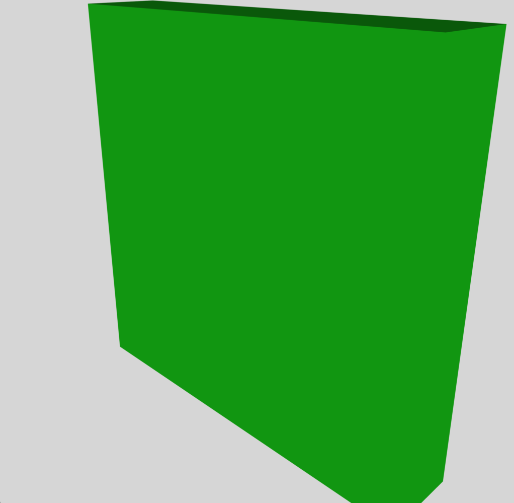
While I was able to view this file successfully within the Preview app on my Mac, it did not display at all on either of the above-identified 3D viewers that I had installed on my Galaxy S8+. As I discovered, the primary issue had to do with how the set of eight vertices were being connected in order to define the model's polygons. In the Example #1 <xml> code, the polygons instruction is used to define six 4-sided polygons. Evidently neither of the Galaxy S8+ viewers understands this polygons instruction. When I used, instead, the triangles instruction to define twelve 3-sided polygons, both of these viewers displayed a 3D object. Here is the relevant, modified executable COLLADA (.dae) file; on my Mac, the filename is: /Dropbox/3Dviewers/Cube/ThirdCube/AppendA08Works.dae

Example #2 — Basically the same as Example #1, but with <triangles> replacing <polygons>

<?xml version="1.0" encoding="utf-8"?>
<COLLADA xmlns="http://www.collada.org/2005/11/COLLADASchema" version="1.4.1">
  <asset>
    <created>2005-11-14T02:16:38Z</created>
    <modified>2005-11-15T11:36:38Z</modified>
    <revision>1.0</revision>
  </asset>
  <library_effects>
    <effect id="whitePhong">
      <profile_COMMON>
        <technique sid="phong1">
          <phong>
            <diffuse>
              <color>0.1 0.9 0.1 1.0</color>
            </diffuse>
          </phong>
        </technique>
      </profile_COMMON>
    </effect>
  </library_effects>
<!--                 -->
  <library_materials>
    <material id="whiteMaterial">
      <instance_effect url="#whitePhong"/>
    </material>
  </library_materials>
  <library_geometries>
    <geometry id="box" name="box">
      <mesh>
        <source id="box-Pos">
          <float_array id="box-Pos-array" count="24">
            0.5  0.5 -0.5
            0.5 -0.5 -0.5
           -0.5 -0.5 -0.5
           -0.5  0.5 -0.5
            0.5  0.5  0.5
            0.5 -0.5  0.5
           -0.5 -0.5  0.5
           -0.5  0.5  0.5
          </float_array>
          <technique_common>
            <accessor source="#box-Pos-array" count="8" stride="3">
              <param name="X" type="float" />
              <param name="Y" type="float" />
              <param name="Z" type="float" />
            </accessor>
          </technique_common>
        </source>
        <source id="box-0-Normal">
          <float_array id="box-0-Normal-array" count="18">
           0.0  0.0 -1.0
           0.0  0.0  1.0
           1.0  0.0  0.0
           0.0 -1.0  0.0
          -1.0  0.0  0.0
           0.0  1.0  0.0
          </float_array>
          <technique_common>
            <accessor source="#box-0-Normal-array" count="6" stride="3">
              <param name="X" type="float"/>
              <param name="Y" type="float"/>
              <param name="Z" type="float"/>
            </accessor>
          </technique_common>
        </source>
        <vertices id="box-Vtx">
          <input semantic="POSITION" source="#box-Pos"/>
        </vertices>
        <triangles count="12" material="WHITE">
          <input semantic="VERTEX" source="#box-Vtx" offset="0"/>
          <input semantic="NORMAL" source="#box-0-Normal" offset="1"/>
          <p>0 0 2 0 3 0   7 1 5 1 4 1   4 2 1 2 0 2   5 3 2 3 1 3   2 4 7 4 3 4   0 5 7 5 4 5   0 0 1 0 2 0   7 1 6 1 5 1   4 2 5 2 1 2   5 3 6 3 2 3   2 4 6 4 7 4   0 5 3 5 7 5</p>
        </triangles>
      </mesh>
    </geometry>
  </library_geometries>
  <library_visual_scenes>
    <visual_scene id="DefaultScene">
      <node id="Box" name="Box">
        <translate> 0  0  3</translate>
        <rotate> 0  0  1  0</rotate>
        <rotate> 0  1  0  0</rotate>
        <rotate> 1  0  0  0</rotate>
        <scale>  1  1  0.2</scale>
        <instance_geometry url="#box">
          <bind_material>
            <technique_common>
              <instance_material symbol="WHITE" target="#whiteMaterial"/>
            </technique_common>
          </bind_material>
        </instance_geometry>
      </node>
    </visual_scene>
  </library_visual_scenes>
  <scene>
    <instance_visual_scene url="#DefaultScene"/>
  </scene>
</COLLADA>

Here are a few additional items of note regarding Example #2:

I set the <color> value to (R, G, B, alpha) = (0.1, 0.9, 0.1, 1), so the resulting "cube" is colored green.
I set the coordinate <scale> factors to (X, Y, Z) = (1, 1, 0.2), so the resulting "cube" is actually a solid rectangle that is substantially flatter in the Z-direction than in the other two directions.
While the Preview app on the Mac and the COLLADA Viewer on the Galaxy S8+ both displayed a flattened, green solid rectangle as depicted here to the right of the Example #2 <xml> model file, the 3D Model Viewer displayed a white cube instead.

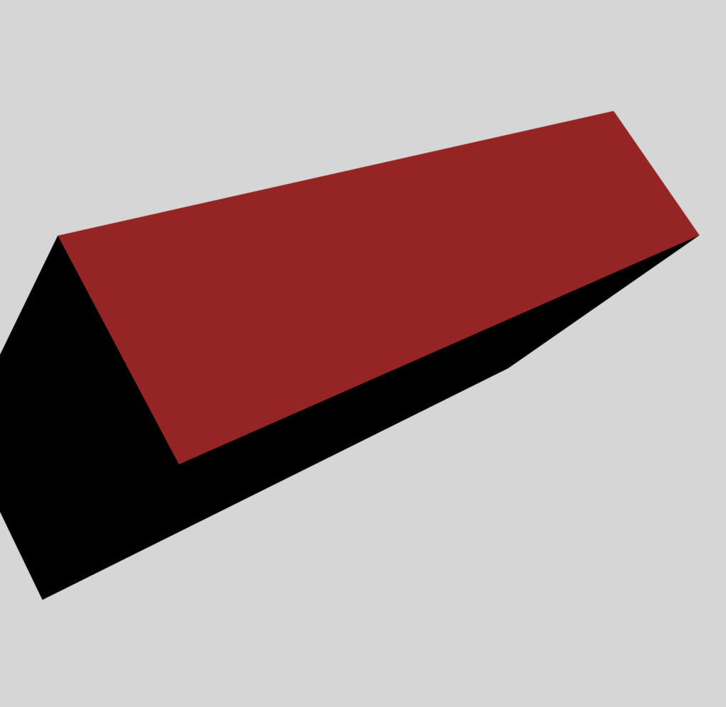
We played with the <xml> code a bit more, changing individual instructions and/or changing various attribute values in an effort to better understand the consequences. The Example #3 <xml> code, shown immediately below, includes many of these alterations; on my Mac the filename is: /Dropbox/3Dviewers/Cube/FourthCube/AppendD13.dae. Both the Preview app on the Mac and the COLLADA Viewer on my Galaxy S8+ generated the red, solid rectangular model depicted here to the right of the Example #3 <xml> model file. The 3D Model Viewer displayed a red, rather than a white, object, which we count as a measure of success; but the displayed 3D object was still an equal-sided cube.

In evolving from the <xml> code displayed here as Example #2 to the <xml> code labeled Example #3, the following two changes appear to have been necessary in order for the 3D Model Viewer to display a red — rather than a white — cube:

In both Example #2 code locations where the attribute "WHITE" appears, we substituted the attribute "whiteMaterial".
In Example #3, the <visual_scene> includes what appears to be a key additional instruction, namely, <matrix sid="transform">.

Example #3 — Basically the same as Example #2, but after playing with various code modifications

<?xml version="1.0" encoding="utf-8"?>
<COLLADA xmlns="http://www.collada.org/2005/11/COLLADASchema" version="1.4.1">
  <asset>
    <created>2005-11-14T02:16:38Z</created>
    <modified>2005-11-15T11:36:38Z</modified>
    <revision>1.0</revision>
    <unit meter="0.0254" name="inch" />
    <up_axis>Z_UP</up_axis>
  </asset>
  <library_effects>
    <effect id="whitePhong">
      <profile_COMMON>
        <technique sid="phong1">
          <phong>
            <diffuse>
              <color>0.8 0.2 0.2 1.0</color>
            </diffuse>
          </phong>
        </technique>
      </profile_COMMON>
    </effect>
  </library_effects>
<!--                 -->
  <library_materials>
    <material id="whiteMaterial">
      <instance_effect url="#whitePhong"/>
    </material>
  </library_materials>
  <library_geometries>
    <geometry id="box" name="box">
      <mesh>
        <source id="box-Pos">
          <float_array id="box-Pos-array" count="24">
            0.0  1.0  1.0
            1.0  1.0  1.0
            0.0  0.0  1.0
            1.0  0.0  1.0
            0.0  1.0  0.0
            1.0  1.0  0.0
            0.0  0.0  0.0
            1.0  0.0  0.0
          </float_array>
          <technique_common>
            <accessor source="#box-Pos-array" count="8" stride="3">
              <param name="X" type="float" />
              <param name="Y" type="float" />
              <param name="Z" type="float" />
            </accessor>
          </technique_common>
        </source>
        <source id="box-0-Normal">
          <float_array id="box-0-Normal-array" count="18">
           1.0  0.0  0.0
          -1.0  0.0  0.0
           0.0  1.0  0.0
           0.0 -1.0  0.0
           0.0  0.0  1.0
           0.0  0.0 -1.0
          </float_array>
          <technique_common>
            <accessor source="#box-0-Normal-array" count="6" stride="3">
              <param name="X" type="float"/>
              <param name="Y" type="float"/>
              <param name="Z" type="float"/>
            </accessor>
          </technique_common>
        </source>
        <vertices id="box-Vtx">
          <input semantic="POSITION" source="#box-Pos"/>
        </vertices>
        <triangles count="12" material="whiteMaterial">
          <input semantic="VERTEX" source="#box-Vtx" offset="0"/>
          <input semantic="NORMAL" source="#box-0-Normal" offset="1"/>
          <p>0 4 2 4 3 4   0 4 3 4 1 4   4 5 5 5 7 5   4 5 7 5 6 5   0 3 4 3 6 3   0 3 6 3 2 3   3 2 7 2 5 2   3 2 5 2 1 2   2 1 6 1 7 1   2 1 7 1 3 1   0 0 1 0 5 0   0 0 5 0 4 0</p>
        </triangles>
<!--
        <polygons count="6" material="whiteMaterial">
          <input semantic="VERTEX" source="#box-Vtx" offset="0"/>
          <input semantic="NORMAL" source="#box-0-Normal" offset="1"/>
          <p>0 4 2 4 3 4 1 4</p>
          <p>0 2 1 2 5 2 4 2</p>
          <p>6 3 7 3 3 3 2 3</p>
          <p>0 1 4 1 6 1 2 1</p>
          <p>3 0 7 0 5 0 1 0</p>
          <p>5 5 7 5 6 5 4 5</p>
        </polygons>
-->
      </mesh>
    </geometry>
  </library_geometries>
  <library_visual_scenes>
    <visual_scene id="DefaultScene">
      <node id="Box" name="Box">
<!--
        <translate> 0  0.5  0.5</translate>
        <rotate> 0  0  0  0</rotate>
        <rotate> 0  0  0  0</rotate>
        <rotate> 0  0  0  0</rotate>
        <scale>  1  0.2  0.1</scale>
        <matrix sid="transform">1 0 0 0 0 0.292 0 0 0 0 1 1.026 0 0 0 1</matrix>
-->
        <rotate> 0  0  1  0</rotate>
        <rotate> 0  1  0  45</rotate>
        <rotate> 1  0  0  0</rotate>
        <scale>  0.05  0.2  0.1</scale>
        <matrix sid="transform">1 0 0 0 0 1 0 0 0 0 1 0 0 0 0 1</matrix>
        <instance_geometry url="#box">
          <bind_material>
            <technique_common>
              <instance_material symbol="whiteMaterial" target="#whiteMaterial"/>
            </technique_common>
          </bind_material>
        </instance_geometry>
      </node>
    </visual_scene>
  </library_visual_scenes>
  <scene>
    <instance_visual_scene url="#DefaultScene"/>
  </scene>
</COLLADA>

Cube Trio by a Blender Developer

Implementing the Raw COLLADA Code

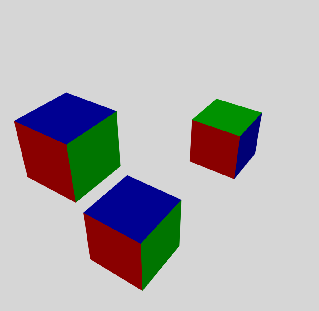
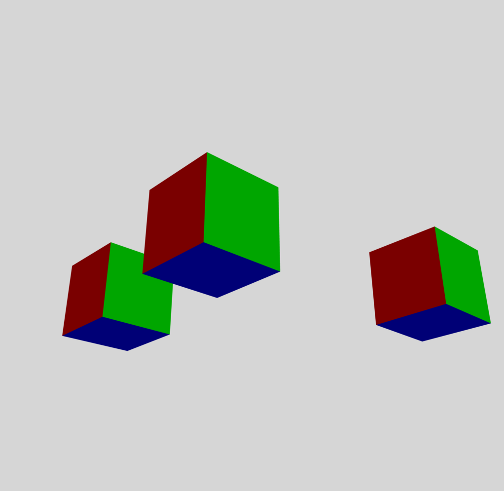
We have found another relatively simple COLLADA-formatted 3D model file on a web page titled, "cube.dae," that has been provided by Blender author, Martjn Berger. The interactive scene that is generated by this model file includes three separate — but identical — cubes; four of the cube faces are painted with one color (e.g., blue), another face is painted with a different color (e.g., green), and the sixth face is painted with yet a different color (e.g., red). The COLLADA-formatted (.dae) file presented immediately below as Example #4 is modified slightly from this original Blender example; on my Mac, the filename is: /Dropbox/3Dviewers/Cube/FirstCube/colladaPlay06.dae

Example #4 — A cube trio, slightly modified from a COLLADA file posted by Blender
<?xml version="1.0" encoding="UTF-8" standalone="no" ?> <COLLADA xmlns="http://www.collada.org/2005/11/COLLADASchema" version="1.4.1"> <asset> <contributor> <authoring_tool>Google SketchUp 8.0.11752</authoring_tool> </contributor> <created>2012-04-27T21:07:03Z</created> <modified>2012-04-27T21:07:03Z</modified> <unit meter="0.0254" name="inch" /> <up_axis>Z_UP</up_axis> </asset> <library_visual_scenes> <visual_scene id="ID1"> <node name="SketchUp"> <node id="ID2" name="instance_0"> <matrix>1 0 0 0 0 1 0 25 0 0 1 0 0 0 0 1</matrix> <instance_node url="#ID3" /> </node> <node id="ID28" name="instance_1"> <matrix>1 0 0 15 0 1 0 120 0 0 1 0 0 0 0 1</matrix> <instance_node url="#ID3" /> </node> <node id="ID29" name="instance_2"> <matrix>1 0 0 120 0 1 0 0 0 0 1 0 0 0 0 1</matrix> <instance_node url="#ID3" /> </node> </node> </visual_scene> </library_visual_scenes> <library_nodes> <node id="ID3" name="cube_component"> <instance_geometry url="#ID4"> <bind_material> <technique_common> <instance_material symbol="Material2" target="#ID6"> <bind_vertex_input semantic="UVSET0" input_semantic="TEXCOORD" input_set="0" /> </instance_material> </technique_common> </bind_material> </instance_geometry> <instance_geometry url="#ID12"> <bind_material> <technique_common> <instance_material symbol="Material2" target="#ID13"> <bind_vertex_input semantic="UVSET0" input_semantic="TEXCOORD" input_set="0" /> </instance_material> </technique_common> </bind_material> </instance_geometry> <instance_geometry url="#ID20"> <bind_material> <technique_common> <instance_material symbol="Material2" target="#ID21"> <bind_vertex_input semantic="UVSET0" input_semantic="TEXCOORD" input_set="0" /> </instance_material> </technique_common> </bind_material> </instance_geometry> </node> </library_nodes> <library_geometries> <geometry id="ID4"> <mesh> <source id="ID7"> <float_array id="ID10" count="48">39.37007874015748 39.37007874015748 0 0 0 0 0 39.37007874015748 0 39.37007874015748 0 0 0 39.37007874015748 39.37007874015748 39.37007874015748 39.37007874015748 0 0 39.37007874015748 0 39.37007874015748 39.37007874015748 39.37007874015748 39.37007874015748 39.37007874015748 0 39.37007874015748 0 39.37007874015748 39.37007874015748 0 0 39.37007874015748 39.37007874015748 39.37007874015748 39.37007874015748 0 39.37007874015748 0 39.37007874015748 39.37007874015748 0 0 39.37007874015748 39.37007874015748 39.37007874015748 39.37007874015748</float_array> <technique_common> <accessor count="16" source="#ID10" stride="3"> <param name="X" type="float" /> <param name="Y" type="float" /> <param name="Z" type="float" /> </accessor> </technique_common> </source> <source id="ID8"> <float_array id="ID11" count="48">0 0 -1 0 0 -1 0 0 -1 0 0 -1 0 1 0 0 1 0 0 1 0 0 1 0 1 0 0 1 0 0 1 0 0 1 0 0 0 0 1 0 0 1 0 0 1 0 0 1</float_array> <technique_common> <accessor count="16" source="#ID11" stride="3"> <param name="X" type="float" /> <param name="Y" type="float" /> <param name="Z" type="float" /> </accessor> </technique_common> </source> <vertices id="ID9"> <input semantic="POSITION" source="#ID7" /> <input semantic="NORMAL" source="#ID8" /> </vertices> <triangles count="8" material="Material2"> <input offset="0" semantic="VERTEX" source="#ID9" /> <p>0 1 2 1 0 3 4 5 6 5 4 7 8 9 10 9 8 11 12 13 14 13 12 15</p> </triangles> </mesh> </geometry> <geometry id="ID12"> <mesh> <source id="ID15"> <float_array id="ID18" count="12">39.37007874015748 0 39.37007874015748 0 0 0 39.37007874015748 0 0 0 0 39.37007874015748</float_array> <technique_common> <accessor count="4" source="#ID18" stride="3"> <param name="X" type="float" /> <param name="Y" type="float" /> <param name="Z" type="float" /> </accessor> </technique_common> </source> <source id="ID16"> <float_array id="ID19" count="12">-0 -1 -0 -0 -1 -0 -0 -1 -0 -0 -1 -0</float_array> <technique_common> <accessor count="4" source="#ID19" stride="3"> <param name="X" type="float" /> <param name="Y" type="float" /> <param name="Z" type="float" /> </accessor> </technique_common> </source> <vertices id="ID17"> <input semantic="POSITION" source="#ID15" /> <input semantic="NORMAL" source="#ID16" /> </vertices> <triangles count="2" material="Material2"> <input offset="0" semantic="VERTEX" source="#ID17" /> <p>0 1 2 1 0 3</p> </triangles> </mesh> </geometry> <geometry id="ID20"> <mesh> <source id="ID23"> <float_array id="ID26" count="12">0 39.37007874015748 39.37007874015748 0 0 0 0 0 39.37007874015748 0 39.37007874015748 0</float_array> <technique_common> <accessor count="4" source="#ID26" stride="3"> <param name="X" type="float" /> <param name="Y" type="float" /> <param name="Z" type="float" /> </accessor> </technique_common> </source> <source id="ID24"> <float_array id="ID27" count="12">-1 0 0 -1 0 0 -1 0 0 -1 0 0</float_array> <technique_common> <accessor count="4" source="#ID27" stride="3"> <param name="X" type="float" /> <param name="Y" type="float" /> <param name="Z" type="float" /> </accessor> </technique_common> </source> <vertices id="ID25"> <input semantic="POSITION" source="#ID23" /> <input semantic="NORMAL" source="#ID24" /> </vertices> <triangles count="2" material="Material2"> <input offset="0" semantic="VERTEX" source="#ID25" /> <p>0 1 2 1 0 3</p> </triangles> </mesh> </geometry> </library_geometries> <library_materials> <material id="ID6" name="material"> <instance_effect url="#ID5" /> </material> <material id="ID13" name="Color_005_"> <instance_effect url="#ID14" /> </material> <material id="ID21" name="Color_A06_"> <instance_effect url="#ID22" /> </material> </library_materials> <library_effects> <effect id="ID5"> <profile_COMMON> <technique sid="COMMON"> <lambert> <diffuse> <color>0 0 1 1</color> </diffuse> </lambert> </technique> </profile_COMMON> </effect> <effect id="ID14"> <profile_COMMON> <technique sid="COMMON"> <lambert> <diffuse> <color>0 1 0 1</color> </diffuse> </lambert> </technique> </profile_COMMON> </effect> <effect id="ID22"> <profile_COMMON> <technique sid="COMMON"> <lambert> <diffuse> <color>0.8 0 0 1</color> </diffuse> </lambert> </technique> </profile_COMMON> </effect> </library_effects> <scene> <instance_visual_scene url="#ID1" /> </scene> </COLLADA>
Principal responsibilities of various subsections from the above, <xml>-formatted code:
A.	<library_visual_scenes> <visual_scene ID="ID1"> <node name="SketcUp"> Generate 3 instances of #ID3, placing them at 3 separate 16-argument "matrix" positions, as explained below. </node> </visual_scene> </library_visual_scenes>
B.	<library_nodes> <node id="ID3"> Define all components of a single node that describes a simple, 6-sided (8 vertices and 12 triangles) cube; this implementation builds the cube as being composed of three separate <instance_geometries>, as defined below: url = "#ID4" should be colored/shaded as defined by material target = "#ID6", which in turn points to library effect = "#ID5". url = "#ID12" should be colored/shaded as defined by material target = "#ID13", which in turn points to library effect = "#ID14". url = "#ID20" should be colored/shaded as defined by material target = "#ID21", which in turn points to library effect = "#ID22". </node> </library_nodes>
C.	<library_geometries> <geometry id="…"> Two co-planar and adjacent triangles are prescribed such that, together, they define a square, which serves as one of the six sides of the cube; four unique vertices are required, referenced as … 0, 1, 2, 3. <mesh> <vertices id="ID17"> (X, Y, Z) coordinate locations are pulled from <source id="ID15"> , which contains a total of 4 × 3 = 12 floating-point numbers. The (X, Y, Z)-normals assigned to the four vertices are pulled from <source id="ID16"> , which also contains a total of 4 × 3 = 12 floating-point numbers … the assigned values are usually 0 or ± 1. </vertices> <triangles source="#ID17" count="2"> <p>0 1 2 1 0 3</p> This sequence of six integers means that the 1^st (of count="2") triangular polygon is formed by connecting three vertices in the order … 0, 1, 2, then back to 0; and the 2^nd (of count="2") triangular polygon is formed by connecting three vertices in the order … 1, 0, 3, then back to 1. </triangles> </mesh> </geometry> </library_geometries>

Understanding the Positioning Matrix

Evidently, the COLLADA language allows you to reposition an object — for example, one of the cubes in this trio — (a) by explicitly specifying the separate instructions to <translate>, <rotate>, and <scale>; or (b) by specifying, in the form of a 4×4 <matrix>, a single instruction that combines all of the others via matrix multiplication.

For example, in COLLADA the instruction, <scale>S_x S_y S_z</scale>, is equivalent to,

M_scale =

S_x	0	0
0	S_y	0
0	0	S_z

And, drawing from the Wikipedia discussion of Basic Rotations in three dimensions, we recognize that rotations about the x, y, and z axes are quantitatively defined, respectively, by the following matrices:

R_x(α) =

1	0	0
0	cos(α)	- sin(α)
0	sin(α)	cos(α)

; R_y(β) =

cos(β)	0	sin(β)
0	1	0
-sin(β)	0	cos(β)

; R_z(γ) =

cos(γ)	- sin(γ)	0
sin(γ)	cos(γ)	0
0	0	1

The equivalent instructions in COLLADA are, respectively,

<rotate> 1 0 0 α </rotate> ;

<rotate> 0 1 0 β </rotate> ;

<rotate> 0 0 1 γ </rotate> .

Drawing furthermore from the Wikipedia discussion of more General Rotations, we recognize that other rotation matrices can be obtained from these three using matrix multiplications. For example, the product

<math>~R(\alpha,\beta,\gamma) = R_z(\alpha) \times R_y(\beta) \times R_x(\gamma) \, ,</math>

— a 3×3 matrix — represents a rotation whose yaw, pitch, and roll angles are α, β, and γ, respectively. Finally, including possible translations T_x, T_y, and T_z in the x, y, and z directions, respectively, we can write

x'

y'

z'

=

T_x

T_y

T_z

+

R(α, β, γ) × M_scale
[3×3 matrix]

×

x

y

z

or, equivalently (I think this is correct!),

x'

y'

z'

1

=

R(α, β, γ) × M_scale			T_x
			T_y
			T_z
0	0	0	1

×

x

y

z

1

Example Implementation

Explicit Specification of Translate and Rotate Instructions

Here we present a COLLADA-formatted (.dae) file that is similar — and in some respects, identical — to the file presented above as Example #4. The new 3D model that is generated by this file consists of three identically colored cubes, as above, but here in Example #5 …

The originating cube is centered on the origin (X,Y,Z) = (0,0,0) of the coordinate system; that is, in the subsection of the .dae file titled, <library_geometries>, each cube edge extends from -20 to + 20 instead of (as in Example #4) from 0 to + 40.
In the subsection of the .dae file titled, <library_vsual_scenes>, the location and orientation of each of the three spawned cubes is determined by the explicit commands, <translate> and <rotate>, instead of (as in Example #4) by the consolidated <matrix> command.

On my Mac, the filename of this Example #5 COLLADA-formatted (.dae) file is: /Dropbox/3Dviewers/Cube/FirstCube/colladaOther20_HBook.dae

Example #5 — Another Cube Trio

<?xml version="1.0" encoding="UTF-8" standalone="no" ?>
<COLLADA xmlns="http://www.collada.org/2005/11/COLLADASchema" version="1.4.1">
    <asset>
        <contributor>
            <authoring_tool>Google SketchUp 8.0.11752</authoring_tool>
        </contributor>
        <created>2012-04-27T21:07:03Z</created>
        <modified>2012-04-27T21:07:03Z</modified>
        <unit meter="0.0254" name="inch" />
        <up_axis>Z_UP</up_axis>
    </asset>
    <library_visual_scenes>
        <visual_scene id="ID1">
            <node name="SketchUp">
                <node id="ID2" name="instance_0">
                    <translate>0.0 45.0 45.0</translate>
                    <instance_node url="#ID3" />
                </node>
                <node id="ID28" name="instance_1">
                    <translate>0.0 0.0 0.0</translate>
                    <instance_node url="#ID3" />
                </node>
                <node id="ID29" name="instance_2">
                    <translate>120.0 0.0 0.0</translate>
                    <rotate> 0 0 1 -90</rotate>
                    <rotate> 1 0 0 -90</rotate>
                    <rotate> 0 1 0 -90</rotate>
<!--  NOTE:  Mac's Preview app excutes these rotations from the bottom (first) to the top (last).
             For example, this one does Y-rot, then X-rot, then Z-rot
-->
                    <instance_node url="#ID3" />
                </node>
            </node>
        </visual_scene>
    </library_visual_scenes>
    <library_nodes>
        <node id="ID3" name="cube_component">
            <instance_geometry url="#ID4">
                <bind_material>
                    <technique_common>
                        <instance_material symbol="Material2" target="#ID6">
                            <bind_vertex_input semantic="UVSET0" input_semantic="TEXCOORD" input_set="0" />
                        </instance_material>
                    </technique_common>
                </bind_material>
            </instance_geometry>
            <instance_geometry url="#ID12">
                <bind_material>
                    <technique_common>
                        <instance_material symbol="Material2" target="#ID13">
                            <bind_vertex_input semantic="UVSET0" input_semantic="TEXCOORD" input_set="0" />
                        </instance_material>
                    </technique_common>
                </bind_material>
            </instance_geometry>
            <instance_geometry url="#ID20">
                <bind_material>
                    <technique_common>
                        <instance_material symbol="Material2" target="#ID21">
                            <bind_vertex_input semantic="UVSET0" input_semantic="TEXCOORD" input_set="0" />
                        </instance_material>
                    </technique_common>
                </bind_material>
            </instance_geometry>
        </node>
    </library_nodes>
    <library_geometries>
        <geometry id="ID4">
            <mesh>
                <source id="ID7">
                    <float_array id="ID10" count="48"> 20.0 20.0 -20.0 -20.0 -20.0 -20.0 -20.0 20.0 -20.0 20.0 -20.0 -20.0 -20.0 20.0 20.0 20.0 20.0 -20.0 -20.0 20.0 -20.0 20.0 20.0 20.0 20.0 20.0 -20.0 20.0 -20.0 20.0 20.0 -20.0 -20.0 20.0 20.0 20.0 20.0 -20.0 20.0 -20.0 20.0 20.0 -20.0 -20.0 20.0 20.0 20.0 20.0</float_array>
                    <technique_common>
                        <accessor count="16" source="#ID10" stride="3">
                            <param name="X" type="float" />
                            <param name="Y" type="float" />
                            <param name="Z" type="float" />
                        </accessor>
                    </technique_common>
                </source>
                <source id="ID8">
                    <float_array id="ID11" count="48">0 0 -1 0 0 -1 0 0 -1 0 0 -1 0 1 0 0 1 0 0 1 0 0 1 0 1 0 0 1 0 0 1 0 0 1 0 0 0 0 1 0 0 1 0 0 1 0 0 1</float_array>
                    <technique_common>
                        <accessor count="16" source="#ID11" stride="3">
                            <param name="X" type="float" />
                            <param name="Y" type="float" />
                            <param name="Z" type="float" />
                        </accessor>
                    </technique_common>
                </source>
                <vertices id="ID9">
                    <input semantic="POSITION" source="#ID7" />
                    <input semantic="NORMAL" source="#ID8" />
                </vertices>
                <triangles count="8" material="Material2">
                    <input offset="0" semantic="VERTEX" source="#ID9" />
                    <p>0 1 2 1 0 3 4 5 6 5 4 7 8 9 10 9 8 11 12 13 14 13 12 15</p>
                </triangles>
            </mesh>
        </geometry>
        <geometry id="ID12">
            <mesh>
                <source id="ID15">
                    <float_array id="ID18" count="12">20.0 -20.0 20.0 -20.0 -20.0 -20.0 20.0 -20.0 -20.0 -20.0 -20.0 20.0</float_array>
                    <technique_common>
                        <accessor count="4" source="#ID18" stride="3">
                            <param name="X" type="float" />
                            <param name="Y" type="float" />
                            <param name="Z" type="float" />
                        </accessor>
                    </technique_common>
                </source>
                <source id="ID16">
                    <float_array id="ID19" count="12">-0 -1 -0 -0 -1 -0 -0 -1 -0 -0 -1 -0</float_array>
                    <technique_common>
                        <accessor count="4" source="#ID19" stride="3">
                            <param name="X" type="float" />
                            <param name="Y" type="float" />
                            <param name="Z" type="float" />
                        </accessor>
                    </technique_common>
                </source>
                <vertices id="ID17">
                    <input semantic="POSITION" source="#ID15" />
                    <input semantic="NORMAL" source="#ID16" />
                </vertices>
                <triangles count="2" material="Material2">
                    <input offset="0" semantic="VERTEX" source="#ID17" />
                    <p>0 1 2 1 0 3</p>
                </triangles>
            </mesh>
        </geometry>
        <geometry id="ID20">
            <mesh>
                <source id="ID23">
                    <float_array id="ID26" count="12">-20.0 20.0 20.0 -20.0 -20.0 -20.0 -20.0 -20.0 20.0 -20.0 20.0 -20.0</float_array>
                    <technique_common>
                        <accessor count="4" source="#ID26" stride="3">
                            <param name="X" type="float" />
                            <param name="Y" type="float" />
                            <param name="Z" type="float" />
                        </accessor>
                    </technique_common>
                </source>
                <source id="ID24">
                    <float_array id="ID27" count="12">-1 0 0 -1 0 0 -1 0 0 -1 0 0</float_array>
                    <technique_common>
                        <accessor count="4" source="#ID27" stride="3">
                            <param name="X" type="float" />
                            <param name="Y" type="float" />
                            <param name="Z" type="float" />
                        </accessor>
                    </technique_common>
                </source>
                <vertices id="ID25">
                    <input semantic="POSITION" source="#ID23" />
                    <input semantic="NORMAL" source="#ID24" />
                </vertices>
                <triangles count="2" material="Material2">
                    <input offset="0" semantic="VERTEX" source="#ID25" />
                    <p>0 1 2 1 0 3</p>
                </triangles>
            </mesh>
        </geometry>
    </library_geometries>
    <library_materials>
        <material id="ID6" name="material">
            <instance_effect url="#ID5" />
        </material>
        <material id="ID13" name="Color_005_">
            <instance_effect url="#ID14" />
        </material>
        <material id="ID21" name="Color_A06_">
            <instance_effect url="#ID22" />
        </material>
    </library_materials>
    <library_effects>
        <effect id="ID5">
            <profile_COMMON>
                <technique sid="COMMON">
                    <lambert>
                        <diffuse>
                            <color>0 0 1 1</color>
                        </diffuse>
                    </lambert>
                </technique>
            </profile_COMMON>
        </effect>
        <effect id="ID14">
            <profile_COMMON>
                <technique sid="COMMON">
                    <lambert>
                        <diffuse>
                            <color>0 1 0 1</color>
                        </diffuse>
                    </lambert>
                </technique>
            </profile_COMMON>
        </effect>
        <effect id="ID22">
            <profile_COMMON>
                <technique sid="COMMON">
                    <lambert>
                        <diffuse>
                            <color>0.8 0 0 1</color>
                        </diffuse>
                    </lambert>
                </technique>
            </profile_COMMON>
        </effect>
    </library_effects>
    <scene>
        <instance_visual_scene url="#ID1" />
    </scene>
</COLLADA>

The 2D, projected image that is shown here to the right of the Example #5 COLLADA code presents the trio of cubes viewed from a particular camera distance and angle. Each of the three cubes is associated with a particular "node" and has been tagged with a unique ID number inside of the subsection of the code titled, <visual_scene>:

ID28 is the node/tag assigned to the cube that appears in the 2D projected image at the bottom-center of the trio; because <translate> X, Y, Z </translate> = <translate> 0.0 0.0 0.0 </translate>, we appreciate that the center of this cube lies at the origin of the 3D coordinate system.
ID2 is the node/tag assigned to the cube that appears in the upper-left position among the trio; according to the relevant <translate> instruction, the center of this cube has been shifted from the coordinate-system origin by 45.0 units in both the Y and Z directions.
ID29 is the node/tag assigned to the cube that appears in the upper-right position among the trio; according to its <translate> instruction, the center of this cube has been shifted from the coordinate-system origin by 120.0 units in the X direction.

From the text of the COLLADA-formatted code (displayed here in the scrolling window of Example #5), we see that in addition to undergoing a translation, the cube tagged with ID29 also has undergone three rotations. As seen in the projected 2D image, the result is that — relative to either one of the other two cubes, which have not undergone rotations — the green face of the cube has effectively swapped positions with a blue cube face. More specifically, here is what has happened to this cube in the 3D model. Reading the three <rotate> instructions from the bottom, up:

(First) the cube was rotated counter-clockwise by 90° about the Y-axis — the red face rolled under the cube and it was replaced with the blue face that was originally on the top of the cube.
(Second) the cube was rotated counter-clockwise by 90° about the X-axis — the green face rolled to the top of the cube and the (previously hidden) red face rolled from under the cube to the position previously occupied by the green face; and the location of the visible blue face remained unchanged.
(Third) the cube was rotated counter-clockwise by 90° about the Z-axis — the red face moved into the position previously occupied by the visible blue face while a separate (previously hidden) blue face rolled into the position previously held by the red face; and the location of the green face remained unchanged.

VERY IMPORTANT NOTE: The ordering of the rotation instructions in three dimensions is critically important. For example, It is not possible to explain the final orientation of the cube tagged with ID29 by reading and carrying out the three <rotate> commands from the top, down.

Equivalent Matrix Instructions

What is the overall <matrix> instruction associated with the position and orientation of each of these three cubes?

For ID28: there are no associated rotation matrices; there is no associated translation; and, by default, the scaling is (S_x,S_y,S_z) = (1, 1, 1). Hence, the relevant 4×4 matrix is,

S_x	0	0	T_x
0	S_y	0	T_y
0	0	S_z	T_z
0	0	0	1

=

1	0	0	0
0	1	0	0
0	0	1	0
0	0	0	1

and the equivalent <matrix> instruction — which results from concatenating the four rows of 4 numbers to create a single row of 16 numbers — should be,

For ID2: there are no associated rotation matrices; the translation vector is (T_x,T_y,T_z) = (0, 45, 45); and, by default, the scaling is (S_x,S_y,S_z) = (1, 1, 1). Hence, the relevant 4×4 matrix is,

S_x	0	0	T_x
0	S_y	0	T_y
0	0	S_z	T_z
0	0	0	1

=

1	0	0	0
0	1	0	45
0	0	1	45
0	0	0	1

and the equivalent <matrix> instruction should be,

For ID29: the translation vector is (T_x,T_y,T_z) = (120, 0, 0); the scaling, as with the other two cubes, is (S_x,S_y,S_z) = (1, 1, 1); and, this time, there is an associated rotation matrix. Specifically, the rotation matrix is,

R(α,β,γ)

=

R_z(-90) × R_x(-90) × R_y(-90)

=

cos(-90)	-sin(-90)	0
sin(-90)	cos(-90)	0
0	0	1

×

1	0	0
0	cos(-90)	-sin(-90)
0	sin(-90)	cos(-90)

×

cos(-90)	0	sin(-90)
0	1	0
-sin(-90)	0	cos(-90)

=

0	+1	0
-1	0	0
0	0	1

×

1	0	0
0	0	+1
0	-1	0

×

0	0	-1
0	1	0
+1	0	0

=

0	+1	0
-1	0	0
0	0	1

×

0	0	-1
+1	0	0
0	-1	0

=

+1	0	0
0	0	+1
0	-1	0

Hence, the relevant 4×4 matrix is,

R(α, β, γ) × M_scale			T_x
			T_y
			T_z
0	0	0	1

=

+1	0	0	120
0	0	+1	0
0	-1	0	0
0	0	0	1

and the equivalent <matrix> instruction should be,

Indeed, we were able to exactly duplicate the cube trio configuration depicted above in the Example #5 projected 2D image when we replaced the lines of code within the <library_visual_scenes> subsection of the Example #5 .dae file with the following lines of code:

    <library_visual_scenes>
        <visual_scene id="ID1">
            <node name="SketchUp">
                <node id="ID2" name="instance_0">
                    <matrix>1 0 0 0 0 1 0 45 0 0 1 45 0 0 0 1</matrix>
                    <instance_node url="#ID3" />
                </node>
                <node id="ID28" name="instance_1">
                    <matrix>1 0 0 0 0 1 0 0 0 0 1 0 0 0 0 1</matrix>
                    <instance_node url="#ID3" />
                </node>
                <node id="ID29" name="instance_2">
                    <matrix>1 0 0 120 0 0 1 0 0 -1 0 0 0 0 0 1</matrix>
                    <instance_node url="#ID3" />
                </node>
            </node>
        </visual_scene>
    </library_visual_scenes>

This demonstrates that, as conjectured above, the location and orientation of each of the three spawned cubes can be specified by using either (A) the explicit commands, <translate> and <rotate>, or (B) the consolidated <matrix> command.

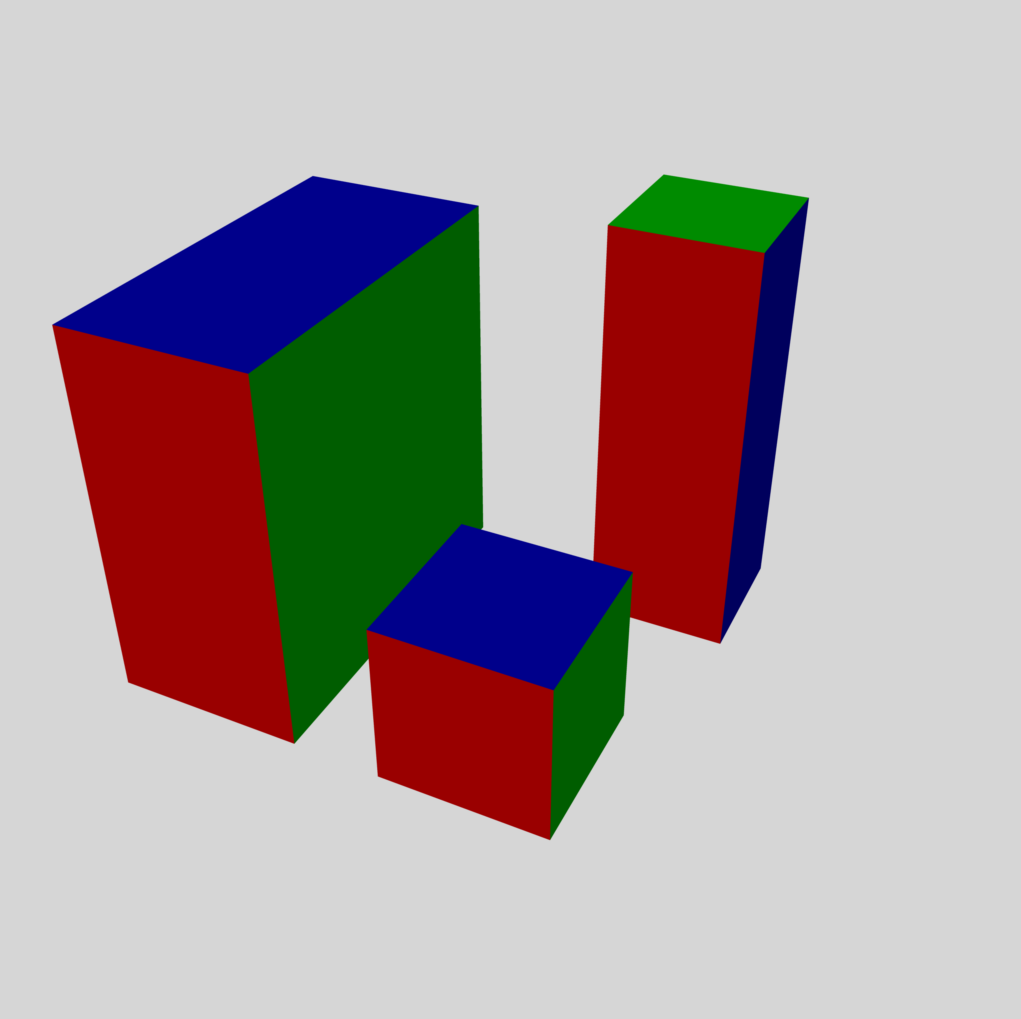
Finally, Example #6 demonstrates how a few small changes in the arguments of the ID2 and ID29 <matrix> commands can change the cubes into, respectively, flattened or elongated solid rectangles.

Example #6 — Incorporating Scaling into <matrix> Commands

    <library_visual_scenes>
        <visual_scene id="ID1">
            <node name="SketchUp">
                <node id="ID2" name="instance_0">
                    <matrix>2 0 0 0 0 1 0 45 0 0 2 45 0 0 0 1</matrix>
                    <instance_node url="#ID3" />
                </node>
                <node id="ID28" name="instance_1">
                    <matrix>1 0 0 0 0 1 0 0 0 0 1 0 0 0 0 1</matrix>
                    <instance_node url="#ID3" />
                </node>
                <node id="ID29" name="instance_2">
                    <matrix>1 0 0 120 0 0 1 0 0 -3 0 0 0 0 0 1</matrix>
                    <instance_node url="#ID3" />
                </node>
            </node>
        </visual_scene>
    </library_visual_scenes>

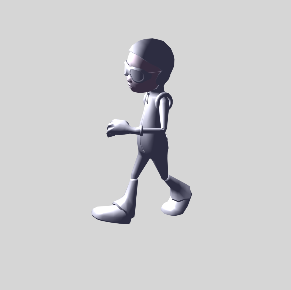
AstroBoyWalk

While searching for an executable COLLADA (.dae) file that illustrates most of the 3D-animation features that I am most interested in and at the same time is relatively simple/short, I came to appreciate that astroBoy_walk is a model that has served as a reasonably good teaching example for the visualization/gaming community over the past ∼decade. I first found the relevant (approximately 5000-line) COLLADA file — named, astroBoy_walk.dae— in a github repository hosted by @jtasn001. Using a repetitive sequence of copy-and-paste strokes — transferring about 60 lines of code at a time — I generated a duplicate of this COLLADA file on my Mac. (Initially, I made one copy/paste mistake; but, thankfully, a second careful perusal through my Mac file identified the error and it was easy to fix.) On my Mac, the filename is: /Dropbox/3Dviewers/astroBoy/JoelBoyWalk02.dae.

Amazingly, when I opened this .dae file inside the Mac's Preview app, a properly constructed 3D astroBoy appeared — absent its associated, colorful texture map. By clicking on/dragging across the Preview window, I was immediately able to view the 3D model from all sides. When I moved the mouse across the lowest segment of the Preview window, a set of stop/play buttons appeared; when I clicked the play button, astroBoy started walking! This was quite exciting, as it meant that in principle I had in-hand a readable & executable COLLADA file that would serve to teach me many essential — and sometimes, subtle — aspects of modern 3D animation/gaming techniques!

NOTE: After joining github on 12 September 2019, I was able to directly download the astroBoy_walk.dae COLLADA file from the @jtasn001 github repository — bypassing the tedious, time-consuming, and error-susceptible copy-and-paste steps. I was also able to directly download from this same repository the boy_10.tga image file that is used by the animation/gaming community as a default, purple & gold texture map for astroBoy. (See Wikipedia's history of .tga file format.)

Immediately below, in the scrolling text window of Example #7, I have highlighted the <xml>-based instructional statements that appear throughout the astroBoy_walk.dae COLLADA file. The results of this initial analysis of the model file should aid my efforts to focus on the visualization tasks that are accomplished in separate, individual subsections of the code.

Example #7 — Initial Analysis of astroBoy_walk.dae

<?xml version="1.0" encoding="utf-8"?>
<COLLADA xmlns="http://www.collada.org/2005/11/COLLADASchema" version="1.4.1">
  <asset>
    <contributor>
      <author>lwong</author>
      <authoring_tool>Maya2008 | ColladaMaya v3.04E</authoring_tool>
      <copyright>
Copyright 2008 Sony Computer Entertainment Inc.
Licensed under the Creative Commons Attribution Noncommercial Share Alike license.
See license file or www.creativecommons.org for details.
      </copyright>
    </contributor>
    <created>2008-06-18T18:16:41Z</created>
    <modified>2008-06-18T18:16:41Z</modified>
    <unit meter="0.01" name="centimeter"/>
    <up_axis>Y_UP</up_axis>
  </asset>
  <library_animations>
    <animation id="spine01.blendParent1"> <!-- Line 21 of 4968 -->
      <source id="spine01.blendParent1_astroBoy_newSkeleton_spine01_blendParent1-input">
        <float_array id="spine01.blendParent1_astroBoy_newSkeleton_spine01_blendParent1-input-array" count="26">
...
      </source>
      <source id="spine01.blendParent1_astroBoy_newSkeleton_spine01_blendParent1-output">
        <float_array id="spine01.blendParent1_astroBoy_newSkeleton_spine01_blendParent1-input-array" count="26">
...
      </source>
      <source id="spine01.blendParent1_astroBoy_newSkeleton_spine01_blendParent1-interpolations">
        <Name_array id="spine01.blendParent1_astroBoy_newSkeleton_spine01_blendParent1-interpolations-array" count="26">
...
      </source>
      <source id="spine01.blendParent1_astroBoy_newSkeleton_spine01_blendParent1-intangents">
        <float_array id="spine01.blendParent1_astroBoy_newSkeleton_spine01_blendParent1-intangents-array" count="52">
...
      </source>
      <source id="spine01.blendParent1_astroBoy_newSkeleton_spine01_blendParent1-outtangents">
        <float_array id="spine01.blendParent1_astroBoy_newSkeleton_spine01_blendParent1-outtangents-array" count="52">
...
      </source>
      <sampler id="spine01.blendParent1_astroBoy_newSkeleton_spine01_blendParent1-sampler">
...
      </sampler>
      <channel source="#spine01.blendParent1_astroBoy_newSkeleton_spine01_blendParent1-sampler" target="astroBoy_newSkeleton_spine01/blendParent1"/>
    </animation> <!-- Line 76 of 4968 -->
...
<!-- Multiple <animation> subsections THRU line #3557 
<animation id="spine01.blendParent1">count = 26, Lines 21 - 76.
<animation id="root.translate">count = 26, Lines 77 - 142
<animation id="root.rotateX">count = 26, Lines 143 - 199
<animation id="root.rotateY">count = 26, Lines 200 - 256
<animation id="root.rotateZ">count = 26, Lines 257 - 314
<animation id="spine01.rotateX">count = 26, Lines 315 - 371
<animation id="spine01.rotateY">count = 26, Lines 372 - 429
<animation id="spine01.rotateZ">count = 26, LInes 430 - 486
<animation id="spine02.rotateX">count = 26, Lines 487 - 543
<animation id="spine02.rotateY">count = 26, Lines 544 - 600
<animation id="spine02.rotateZ">count = 26, Lines 601 - 658
<animation id="neck01.rotateX">count = 26, Lines 659 - 715
<animation id="neck01.rotateY">count = 26, Lines 716 - 772
<animation id="neck01.rotateZ">count = 26, Lines 773 - 829
<animation id="head.rotateX">count = 26, Lines 830 - 886
<animation id="head.rotateY">count = 26, Lines 887 - 944
<animation id="head.rotateZ">count = 26, Lines 945 - 1001
<animation id="L_clavicle.rotateX">count = 26, Lines 1002 - 1058
<animation id="L_clavicle.rotateY">count = 26, Lines 1059 - 1115
<animation id="L_clavicle.rotateZ">count = 26, Lines 1116 - 1173
<animation id="L_shoulder.rotateX">count = 26, Lines 1174 - 1230
<animation id="L_shoulder.rotateY">count = 26, Lines 1231 - 1287
<animation id="L_shoulder.rotateZ">count = 26, Lines 1288 - 1344
<animation id="L_elbow.rotateX">count = 26, Lines 1345 - 1401
<animation id="L_elbow.rotateY">count = 26, Lines 1402 - 1459
<animation id="L_elbow.rotateZ">count = 26, Lines 1460 - 1516
<animation id="L_wrist.rotateZ">count = 26, Lines 1517 - 1573
<animation id="R_clavicle.rotateX">count = 26, Lines 1574 - 1630
<animation id="R_clavicle.rotateY">count = 26, Lines 1631 - 1688
<animation id="R_clavicle.rotateZ">count = 26, Lines 1689 - 1745
<animation id="R_shoulder.rotateX">count = 26, Lines 1746 - 1802
<animation id="R_shoulder.rotateY">count = 26, Lines 1803 - 1859
<animation id="R_shoulder.rotateZ">count = 26, Lines 1860 - 1917
<animation id="R_elbow.rotateX">count = 26, Lines 1918 - 1974
<animation id="R_elbow.rotateY">count = 26, Lines 1975 - 2031
<animation id="R_elbow.rotateZ">count = 26, Lines 2032 - 2088
<animation id="R_wrist.rotateX">count = 26, Lines 2089 - 2146
<animation id="R_wrist.rotateZ">count = 26, Lines 2147 - 2203
<animation id="hips.rotateX"> THRU <animation id="hips.rotateZ">count = 26, Lines 2204 - 2375
<animation id="L_hip.rotateX"> THRU <animation id="L_hip.rotateZ">count = 26, Lines 2376 - 2546
<animation id="L_knee_01.rotateZ">count = 26, Lines 2547 - 2603
<animation id="L_knee_02.rotateZ">count = 26, Lines 2604 - 2661
<animation id="L_ankle.rotateX">  THRU <animation id="L_ankle.rotateZ">count = 26, Lines 2662 - 2832
<animation id="L_toeBall.rotateX"> THRU <animation id="L_toeBall.rotateZ">count = 26, Lines 2833 - 3004
<animation id="R_hip.rotateX"> THRU <animation id="R_hip.rotateZ">count = 26, Lines 3005 - 3176
<animation id="R_knee_01.rotateZ">count = 26, LInes 3177 - 3233
<animation id="R_knee_02.rotateZ">count = 26, Lines 3234 - 3290
<animation id="R_ankle.rotateX"> THRU <animation id="R_ankle.rotateZ">count = 26, Lines 3291 - 3462
<animation id="R_toeBall.rotateX"> THRU <animation id="R_toeBall.rotateZ">count = 26, Lines 3463 - 3634
-->
...
    </animation>
  </library_animations>
  <library_physics_scenes> <!-- Line 3637 of 4968 -->
    <physics_scene id="MayaNativePhysicsScene">
      <technique_common>
        <gravity>0 -980 0</gravity>
        <time_step>0.083</time_step>
      </technique_common>
    </physics_scene>
  </library_physics_scenes>
  <library_lights>
    <light ... pointLightShape1 ...>
    </light>
    <light ... ambientLightShape1 ...>
    </light>
  </library_lights>
  <library_images>
    <image id="file9" name="file9">
      ...
    </image>
  </library_images><!-- THRU line 3687 -->
  <library_materials>
...
  </library_materials>
  <library_effects>
    <effect id="matte-fx">
...
    </effect><!-- THRU line 3782 -->
    <effect id="shiny-fx">
...
    </effect><!-- THRU line 3861 -->
    <effect id="face-fx">
...
    </effect><!-- THRU line 3940 -->
    <effect id="glass-fx">
...
    </effect><!-- THRU line 4019 -->
  </library_effects>
<library_geometries>
    <geometry id="boyShape" name="boyShape">
      <mesh> 
        <source id="boyShape-positions" name="position">
          <float_array id="boyShape-positions-array" count = "7857">                        <!--    3 x 2619 = 7857   -->
          <technique_common>
            <accessor source="#boyShape-positions-array" count="2619" stride="3">
              <param name="X" type="float"/>
              <param name="Y" type="float"/>
              <param name="Z" type="float"/>
            </accessor>
          </technique_common>
        </source>
        <source id="boyShape-normals" name="normal">
          <float_array id="boyShape-normals-array" count="9519">                           <!--    3 x 3173 = 9519   -->
          <technique_common>
            <accessor source="#boyShape-normals-array" count="3173" stride="3">
              <param name="X" type="float"/>
              <param name="Y" type="float"/>
              <param name="Z" type="float"/>
            </accessor>
          </technique_common>
        </source>
        <source id="boyShape-map1" name="map1">
          <float_array id="boyShape-map1-array" count="6444">                              <!--    3 x 2148 = 6444   -->
          <technique_common>
            <accessor source="#boyShape-map1-array" count="3222" stride="2">
              <param name="S" type="float"/>
              <param name="T" type="float"/>
            </accessor>
          </technique_common>
        </source>
        <vertices id="boyShape-vertices">
          <input semantic="POSITION" source="#boyShape-positions"/>
        </vertices>                                                                                                           <!--  Line 4056  -->
        <polylist material="faceSG" count="508">
          <input semantic="VERTEX" source="#boyShape-vertices" offset="0"/>
          <input semantic="NORMAL" source="#boyShape-normals" offset="1"/>
          <input semantic="TEXCOORD" source="#boyShape-map1" offset="2" set="0"/>
          <vcount>
...
          </vcount>
          <p>
...
          </p>
        </polylist>
        <polylist material="glassSG" count="12">
          <input semantic="VERTEX" source="#boyShape-vertices" offset="0"/>
          <input semantic="NORMAL" source="#boyShape-normals" offset="1"/>
          <input semantic="TEXCOORD" source="#boyShape-map1" offset="2" set="0"/>
          <vcount>4 4 4 4 4 4 4 4 4 4 4 4</vcount>
          <p>
...
          </p>
        </polylist>
        <polylist material="shinnySG" count="1454">
          <input semantic="VERTEX" source="#boyShape-vertices" offset="0"/>
          <input semantic="NORMAL" source="#boyShape-normals" offset="1"/>
          <input semantic="TEXCOORD" source="#boyShape-map1" offset="2" set="0"/>
          <vcount>
...
          </vcount>
          <p>
...
          </p>
        </polylist>
        <polylist material="matteSG" count="574">
          <input semantic="VERTEX" source="#boyShape-vertices" offset="0"/>
          <input semantic="NORMAL" source="#boyShape-normals" offset="1"/>
          <input semantic="TEXCOORD" source="#boyShape-map1" offset="2" set="0"/>
          <vcount>
...
          </vcount>
          <p>
...
          </p>
        </polylist>
      </mesh>
      <extra>
...
      </extra>
    </geometry>
  </library_geometries>                                 <!--   THRU line 4103   -->
  <library_controllers>
    <controller id="boyShape-skin" name="skinCluster1">
      <skin source="#boyShape">
        <bind_shape_matrix>1 0 0 0 0 1 0 0 0 0 1 0 0 0 0 1</bind_shape_matrix>
        <source id="boyShape-skin-joints">
...
        </source>
        <source id="boyShape-skin-bind_poses">
...
        </source>
        <source id="boyShape-skin-bind_poses">
          <float_array id="boyShape-skin-bind_poses-array" count="704">
...
          </float_array>
...
        </source>
        <source id="boyShape-skin-weights">
          <float_array id="boyShape-skin-weights-array" count="1160">
...
          </float_array>
...
        </source>
        <joints>
          <input semantic="JOINT" source="#boyShape-skin-joints"/>
          <input semantic="INV_BIND_MATRIX" source="#boyShape-skin-bind_poses"/>
        </joints>
        <vertex_weights count="2619">
          <input semantic="JOINT" source="#boyShape-skin-joints" offset="0"/>
          <input semantic="WEIGHT" source="#boyShape-skin-weights" offset="1"/>
          <vcount> ... </vcounts>
          <v> ... </v>
        </vertex_weights>
      </skin>
    </controller>
  </library_controllers>                                                        <!--   THRU line 4147   -->
  <library_visual_scenes>
    <visual_scene id="VisualSceneNode" name="astroBoy_walkbake">
...
<!-- LOTS OF COMMANDS -->
...
      </visual_scene>
    </library_visual_scenes>                                                        <!--   THRU line 4960   -->
  <scene>
    <instance_physics_scene url="#MayaNativePhysicsScene"/>
    <instance_visual_scene url="#VisualSceneNode"/>
  </scene>
</COLLADA>

Here are a few additional items of note regarding Example #5:

Check out …

Part 1 of Step by Step Skeletal Animation in C++ and OpenGL, Using COLLADA (circa 2010)
Part 2 of Step by Step Skeletal Animation in C++ and OpenGL, Using COLLADA (circa 2010) — especially the subsection titled, "How skeletal Animation Works?"

Clock

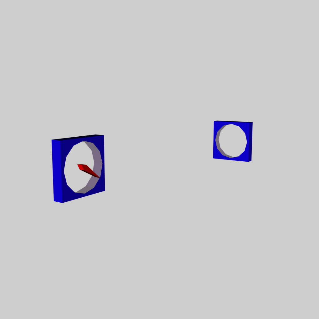
On 23 September 2019 I found, and downloaded from GitHub, a useful COLLADA file — animated-blender-cube.dae, developed by user "chinedufn" — that performs a simple animation of a cube. I successfully replaced the single, grey cube in chinedufn's model with my multi-colored "cube trio" then, calling upon the skills that I had acquired by playing with the astro_boy model, I used this modified animated-cube file to get more comfortable with COLLADA's animation instructions. With this improved understanding, I started from scratch and built a model of a clock entirely within the COLLADA language. This executable .dae file is presented immediately below as Example #8. This model works wonderfully when displayed by my Mac's Preview app.

Example #8 — Our Constructed Model of a Clock

<?xml version="1.0" encoding="utf-8"?>
<COLLADA xmlns="http://www.collada.org/2005/11/COLLADASchema" version="1.4.1">
<!--
On 23 September 2019 I copied the following cube-animation file from github:
https://github.com/chinedufn/collada-dae-parser/blob/master/test/fixture/animated-blender-cube.dae
I have made substantial modifications in order to better understand how the animation instructions
actually work.

THIS FILE NAME:  Dropbox/3Dviewers/Clock/Arrow07.PERFECT.dae
It uses "polylist" and correct implementation of "normals" for all polygons of the Clock.
It also displays **two** clocks:  [Initially, we made one spin and the other not.]
It also adds a red "minute hand" to the clock; now, this is the only segment that spins.
-->
  <asset>
    <contributor>
      <author>jet53man</author>
      <authoring_tool>Raw XML</authoring_tool>
    </contributor>
    <created>2019-09-24</created>
    <modified>2019-09-29</modified>
    <unit name="meter" meter="1"/>
    <up_axis>Z_UP</up_axis>
  </asset>
  <library_images/>
    <library_effects>
        <effect id="ID5">
            <profile_COMMON>
                <technique sid="COMMON">
                    <lambert>
                        <diffuse>
                            <color>0 0 1 1</color>
                        </diffuse>
                    </lambert>
                </technique>
            </profile_COMMON>
        </effect>
        <effect id="InnerID5">
            <profile_COMMON>
                <technique sid="COMMON">
                    <lambert>
                        <diffuse>
                            <color>0.4 0.0 0.7 0.4</color>
                        </diffuse>
                    </lambert>
                </technique>
            </profile_COMMON>
        </effect>
        <effect id="ArrowID5">
            <profile_COMMON>
                <technique sid="COMMON">
                    <lambert>
                        <diffuse>
                            <color>1.0 0.0 0.0 1.0</color>
                        </diffuse>
                    </lambert>
                </technique>
            </profile_COMMON>
        </effect>
    </library_effects>
    <library_materials>
        <material id="ID6" name="material">
            <instance_effect url="#ID5" />
        </material>
        <material id="InnerID6" name="Inner_material">
            <instance_effect url="#InnerID5" />
        </material>
        <material id="ArrowID6" name="Arrow_material">
            <instance_effect url="#ArrowID5" />
        </material>
    </library_materials>
    <library_nodes>
        <node id="ID3" name="cube_component">
            <instance_geometry url="#Clock_OuterEdge">
                <bind_material>
                    <technique_common>
                        <instance_material symbol="Material2" target="#ID6">
                            <bind_vertex_input semantic="UVSET0" input_semantic="TEXCOORD" input_set="0" />
                        </instance_material>
                    </technique_common>
                </bind_material>
            </instance_geometry>
            <instance_geometry url="#Clock_InnerEdge">
                <bind_material>
                    <technique_common>
                        <instance_material symbol="Material2" target="#InnerID6">
                            <bind_vertex_input semantic="UVSET0" input_semantic="TEXCOORD" input_set="0" />
                        </instance_material>
                    </technique_common>
                </bind_material>
            </instance_geometry>
        </node>
        <node id="ArrowID3" name="cube_component">
            <instance_geometry url="#Clock_ArrowEdge">
                <bind_material>
                    <technique_common>
                        <instance_material symbol="Material2" target="#ArrowID6">
                            <bind_vertex_input semantic="UVSET0" input_semantic="TEXCOORD" input_set="0" />
                        </instance_material>
                    </technique_common>
                </bind_material>
            </instance_geometry>
        </node>
    </library_nodes>
    <library_geometries>
        <geometry id="Clock_OuterEdge">
            <mesh>
<!--
            **********************************************
            *
            *  Insert first portion of clock's structure
            *
            **********************************************
-->
                <source id="Clock_Positions">
                  <float_array id="Coordinates01" count="123"> 0.0  1.0  0.2 1.0  1.0  0.2 1.0  0.0  0.2 1.0 -1.0  0.2 0.0 -1.0  0.2 -1.0 -1.0  0.2 -1.0  0.0  0.2 -1.0  1.0  0.2 0.0  1.0 -0.2 1.0  1.0 -0.2 1.0  0.0 -0.2 1.0 -1.0 -0.2 0.0 -1.0 -0.2 -1.0 -1.0 -0.2 -1.0  0.0 -0.2 -1.0  1.0 -0.2 0.9  0.0  0.2 0.779423 0.45 0.2 0.45 0.779423 0.2 0.0  0.9  0.2 -0.45 0.779423 0.2 -0.779423 0.45 0.2 -0.9 0.0 0.2 -0.779423 -0.45 0.2 -0.45 -0.779423 0.2 0.0 -0.9 0.2 0.45 -0.779423 0.2 0.779423 -0.45 0.2 -0.9  0.0  -0.2 -0.779423 0.45 -0.2 -0.45 0.779423 -0.2 -0.0  0.9  -0.2 0.45 0.779423 -0.2 0.779423 0.45 -0.2 0.9 0.0 -0.2 0.779423 -0.45 -0.2 0.45 -0.779423 -0.2 -0.0 -0.9 -0.2 -0.45 -0.779423 -0.2 -0.779423 -0.45 -0.2  0.0 0.0 -0.2</float_array>
                  <technique_common>
                    <accessor source="#Coordinates01" count="41" stride="3">
                            <param name="X" type="float" />
                            <param name="Y" type="float" />
                            <param name="Z" type="float" />
                    </accessor>
                  </technique_common>
                </source>
                <source id="Clock_Normals">
                  <float_array id="InnerNormals01" count="18">
 1.0  0.0  0.0
-1.0  0.0  0.0
 0.0  1.0  0.0
 0.0 -1.0  0.0
 0.0  0.0  1.0
 0.0  0.0 -1.0
                  </float_array>
                    <technique_common>
                        <accessor source="#Normals01" count="6" stride="3">
                            <param name="X" type="float" />
                            <param name="Y" type="float" />
                            <param name="Z" type="float" />
                        </accessor>
                    </technique_common>
                </source>
                <vertices id="Clock_Vertices">
                    <input semantic="POSITION" source="#Clock_Positions" />
                </vertices>
                <polylist count="56" material="Material2">
                    <input semantic="VERTEX" source="#Clock_Vertices" offset="0" />
                    <input semantic="NORMAL" source="#Clock_Normals" offset="1" />
<vcount> 3 3 3 3 3  3 3 3 3 3  3 3 3 3 3  3 3 3 3 3  3 3 3 3 3  3 3 3 3 3  3 3 3 3 3  3 3 3 3 3  3 3 3 3 3  3 3 3 3 3  3 3 3 3 3  3</vcount>
<p> 0 2 1 2 8 2  1 2 9 2 8 2  7 2 0 2 15 2  0 2 8 2 15 2 1 0 2 0 9 0  2 0 10 0 9 0  2 0 3 0 10 0  3 0 11 0 10 0 3 3 4 3 11 3  4 3 12 3 11 3  4 3 5 3 12 3  5 3 13 3 12 3 5 1 6 1 13 1  6 1 14 1 13 1  6 1 7 1 14 1  7 1 15 1 14 1 2 4 17 4 16 4  2 4 1 4 17 4  1 4 18 4 17 4  1 4 0 4 18 4  0 4 19 4 18 4 0 4 20 4 19 4  0 4 7 4 20 4  7 4 21 4 20 4  7 4 6 4 21 4  6 4 22 4 21 4 6 4 23 4 22 4  6 4 5 4 23 4  5 4 24 4 23 4  5 4 4 4 24 4  4 4 25 4 24 4 4 4 26 4 25 4  4 4 3 4 26 4  3 4 27 4 26 4  3 4 2 4 27 4  2 4 16 4 27 4 14 5 29 5 28 5  14 5 15 5 29 5  15 5 30 5 29 5  15 5 8 5 30 5  8 5 31 5 30 5 8 5 32 5 31 5  8 5 9 5 32 5  9 5 33 5 32 5  9 5 10 5 33 5  10 5 34 5 33 5 10 5 35 5 34 5  10 5 11 5 35 5  11 5 36 5 35 5  11 5 12 5 36 5  12 5 37 5 36 5 12 5 38 5 37 5  12 5 13 5 38 5  13 5 39 5 38 5  13 5 14 5 39 5  14 5 28 5 39 5 </p>
                </polylist>
            </mesh>
        </geometry>
        <geometry id="Clock_InnerEdge">
            <mesh>
<!--
            **********************************************
            *
            *  Insert second portion of clock's structure
            *
            **********************************************
-->
                <source id="Clock_InnerPositions">
                  <float_array id="InnerCoordinates01" count="123">
0.0  1.0  0.2 1.0  1.0  0.2 1.0  0.0  0.2 1.0 -1.0  0.2 0.0 -1.0  0.2 -1.0 -1.0  0.2 -1.0  0.0  0.2 -1.0  1.0  0.2 0.0  1.0 -0.2 1.0  1.0 -0.2 1.0  0.0 -0.2 1.0 -1.0 -0.2 0.0 -1.0 -0.2 -1.0 -1.0 -0.2 -1.0  0.0 -0.2 -1.0  1.0 -0.2 0.9  0.0  0.2 0.779423 0.45 0.2 0.45 0.779423 0.2 0.0  0.9  0.2 -0.45 0.779423 0.2 -0.779423 0.45 0.2 -0.9 0.0 0.2 -0.779423 -0.45 0.2 -0.45 -0.779423 0.2 0.0 -0.9 0.2 0.45 -0.779423 0.2 0.779423 -0.45 0.2 -0.9  0.0  -0.2 -0.779423 0.45 -0.2 -0.45 0.779423 -0.2 -0.0  0.9  -0.2 0.45 0.779423 -0.2 0.779423 0.45 -0.2 0.9 0.0 -0.2 0.779423 -0.45 -0.2 0.45 -0.779423 -0.2 -0.0 -0.9 -0.2 -0.45 -0.779423 -0.2 -0.779423 -0.45 -0.2  0.0 0.0 -0.2</float_array>
                  <technique_common>
                    <accessor source="#InnerCoordinates01" count="41" stride="3">
                            <param name="X" type="float" />
                            <param name="Y" type="float" />
                            <param name="Z" type="float" />
                    </accessor>
                  </technique_common>
                </source>
                <source id="Clock_InnerNormals">
                  <float_array id="InnerNormals01" count="54">
 1.0  0.0  0.0
-1.0  0.0  0.0
 0.0  1.0  0.0
 0.0 -1.0  0.0
 0.0  0.0  1.0
 0.0  0.0 -1.0
 -0.965926 -0.258819 0.0
 -0.707107 -0.707107 0.0
 -0.258819 -0.965926 0.0
  0.258819 -0.965926 0.0
  0.707107 -0.707107 0.0
  0.965926 -0.258819 0.0
  0.965926  0.258819 0.0
  0.707107  0.707107 0.0
  0.258819  0.965926 0.0
 -0.258819  0.965926 0.0
 -0.707107  0.707107 0.0
 -0.965926  0.258819 0.0
                  </float_array>
                    <technique_common>
                        <accessor source="#InnerNormals01" count="18" stride="3">
                            <param name="X" type="float" />
                            <param name="Y" type="float" />
                            <param name="Z" type="float" />
                        </accessor>
                    </technique_common>
                </source>
                <vertices id="Clock_InnerVertices">
                    <input semantic="POSITION" source="#Clock_InnerPositions" />
                </vertices>
                <polylist count="24" material="Material2">
                    <input semantic="VERTEX" source="#Clock_InnerVertices" offset="0" />
                    <input semantic="NORMAL" source="#Clock_InnerNormals" offset="1"/>
<vcount>4 4 4 4  4 4 4 4  4 4 4 4  3 3 3 3  3 3 3 3  3 3 3 3</vcount>
<p> 16 6 17 6 33 6 34 6 17 7 18 7 32 7 33 7 18 8 19 8 31 8 32 8 19 9 20 9 30 9 31 9 20 10 21 10 29 10 30 10 21 11 22 11 28 11 29 11 22 12 23 12 39 12 28 12 23 13 24 13 38 13 39 13 24 14 25 14 37 14 38 14 25 15 26 15 36 15 37 15 26 16 27 16 35 16 36 16 27 17 16 17 34 17 35 17 28 5 29 5 40 5 29 5 30 5 40 5 30 5 31 5 40 5 31 5 32 5 40 5 32 5 33 5 40 5 33 5 34 5 40 5 34 5 35 5 40 5 35 5 36 5 40 5 36 5 37 5 40 5 37 5 38 5 40 5 38 5 39 5 40 5 39 5 28 5 40 5 </p>
              </polylist>
            </mesh>
        </geometry>
        <geometry id="Clock_ArrowEdge">
            <mesh>
<!--
            **********************************************
            *
            *  Insert arrow portion of clock's structure
            *
            **********************************************
-->
                <source id="Clock_ArrowPositions">
                  <float_array id="ArrowCoordinates01" count="30"> 0.0  0.85 0.25 0.1  0.0 0.25 0.0 -0.2 0.25 -0.1  0.0 0.25 0.0  0.85 0.05 0.1  0.0 0.05 0.0 -0.2 0.05 -0.1  0.0 0.05 0.0  0.0 0.25 0.0  0.0 0.05 </float_array>
                  <technique_common>
                    <accessor source="#ArrowCoordinates01" count="10" stride="3">
                            <param name="X" type="float" />
                            <param name="Y" type="float" />
                            <param name="Z" type="float" />
                    </accessor>
                  </technique_common>
                </source>
                <source id="Clock_ArrowNormals">
                  <float_array id="ArrowNormals01" count="18">
 0  0  1
 0  0 -1
 0.993151  0.116841 0.0
 0.447214 -0.894427 0.0
-0.447214 -0.894427 0.0
-0.993151  0.116841 0.0
                  </float_array>
                    <technique_common>
                        <accessor source="#ArrowNormals01" count="6" stride="3">
                            <param name="X" type="float" />
                            <param name="Y" type="float" />
                            <param name="Z" type="float" />
                        </accessor>
                    </technique_common>
                </source>
                <vertices id="Clock_ArrowVertices">
                    <input semantic="POSITION" source="#Clock_ArrowPositions" />
                </vertices>
                <polylist count="12" material="Material2">
                    <input semantic="VERTEX" source="#Clock_ArrowVertices" offset="0" />
                    <input semantic="NORMAL" source="#Clock_ArrowNormals" offset="1"/>
<vcount>3 3 3 3 3 3 3 3 4 4 4 4</vcount>
<p> 0 0 8 0 1 0 1 0 8 0 2 0 2 0 8 0 3 0 3 0 8 0 0 0 4 1 5 1 9 1 5 1 6 1 9 1 6 1 7 1 9 1 7 1 4 1 9 1 0 2 1 2 5 2 4 2 1 3 2 3 6 3 5 3 2 4 3 4 7 4 6 4 3 5 0 5 4 5 7 5 </p>
              </polylist>
            </mesh>
        </geometry>
    </library_geometries>
  <library_animations>
    <animation id="Cube_rotation_euler_Z">
      <source id="Cube_rotation_euler_Z-input">
<!--        <float_array id="Cube_rotation_euler_Z-input-array" count="5">0 0.2083333 0.4166666 0.625 0.8333333</float_array> -->
<!--        <float_array id="Cube_rotation_euler_Z-input-array" count="5">0 0.4167 0.8333 1.25 1.666</float_array> -->
        <float_array id="Cube_rotation_euler_Z-input-array" count="17">0 0.25 0.5 0.75 1.0 1.25 1.5 1.75 2.0 2.25 2.5 2.75 3.0 3.25 3.5 3.75 4.0</float_array>
        <technique_common>
          <accessor source="#Cube_rotation_euler_Z-input-array" count="5" stride="1">
            <param name="TIME" type="float"/>
          </accessor>
        </technique_common>
      </source>
      <source id="Cube_rotation_euler_Z-output">
<!--        <float_array id="Cube_rotation_euler_Z-output-array" count="5">0 -22.5 -45 -67.5 -90</float_array> -->
        <float_array id="Cube_rotation_euler_Z-output-array" count="17">0 -22.5 -45 -67.5 -90 -112.5 -135.0 -157.5 -180.0 -202.5 -225.0 -247.5 -270.0 -292.5 -315.0 -337.5 -360.0</float_array>
        <technique_common>
          <accessor source="#Cube_rotation_euler_Z-output-array" count="5" stride="1">
            <param name="ANGLE" type="float"/>
          </accessor>
        </technique_common>
      </source>
      <sampler id="Cube_rotation_euler_Z-sampler">
        <input semantic="INPUT" source="#Cube_rotation_euler_Z-input"/>
        <input semantic="OUTPUT" source="#Cube_rotation_euler_Z-output"/>
      </sampler>
      <channel source="#Cube_rotation_euler_Z-sampler" target="jetman/rotationZ.ANGLE"/>
    </animation>
    <animation id="Cube_scale_Z">
      <source id="Cube_scale_Z-input">
<!--        <float_array id="Cube_scale_Z-input-array" count="5">0 0.2083333 0.4166666 0.625 0.8333333</float_array>  -->
        <float_array id="Cube_scale_Z-input-array" count="5">0 0.0694 0.1389 0.2083 0.2778</float_array>
        <technique_common>
          <accessor source="#Cube_scale_Z-input-array" count="5" stride="1">
            <param name="TIME" type="float"/>
          </accessor>
        </technique_common>
      </source>
      <source id="Cube_scale_Z-output">
<!--    <float_array id="Cube_scale_Z-output-array" count="5">0.5 0.4 0.3 0.2 0.1</float_array>  -->
        <float_array id="Cube_scale_Z-output-array" count="5">1.0 1.0 1.0 1.0 1.0</float_array>
        <technique_common>
          <accessor source="#Cube_scale_Z-output-array" count="5" stride="1">
            <param name="Z" type="float"/>
          </accessor>
        </technique_common>
      </source>
      <sampler id="Cube_scale_Z-sampler">
        <input semantic="INPUT" source="#Cube_scale_Z-input"/>
        <input semantic="OUTPUT" source="#Cube_scale_Z-output"/>
      </sampler>
      <channel source="#Cube_scale_Z-sampler" target="jetman/scale.Z"/>
    </animation>
  </library_animations>
    <library_controllers/>
    <library_visual_scenes>
        <visual_scene id="EntireLayout">
<!--
***********
*
* Evidently, it is important for the "id" of this node to be shared
* with the "directory" name that is used in the animation "channel"
* instructions.  For example, "jetman" is used here.
*
***********
-->
          <node id="TwoClocks">
            <node id="firstclock" name="instance_1">
              <translate>0.0 1.0 0.0</translate>
              <rotate sid="rotationX">1 0 0 90</rotate>
              <rotate sid="rotationZ">0 0 1 0</rotate>
<!--
              <rotate sid="rotationY">0 1 0 90</rotate>
-->
              <scale sid="scale">1 1 1</scale>
              <instance_node url="#ID3" />
            </node>
            <node id="jetman" name="instance_Arrow">
              <translate>0.0 1.0 0.0</translate>
              <rotate sid="rotationX">1 0 0 90</rotate>
              <rotate sid="rotationZ">0 0 1 0</rotate>
<!--
              <rotate sid="rotationY">0 1 0 90</rotate>
-->
              <scale sid="scale">1 1 1</scale>
              <instance_node url="#ArrowID3" />
            </node>
            <extra>
              <technique profile="FCOLLADA">
                <start_time>0</start_time>
                <end_time>4.0</end_time>
              </technique>
            </extra>
            <node id="secondClock" name="instance_2">
              <translate>10.0 0.0 0.0</translate>
<!--
              <rotate sid="rotationZ">0 0 1 90</rotate>
-->
              <rotate sid="rotationX">1 0 0 90</rotate>
              <rotate sid="rotationY">0 1 0 -90</rotate>
              <scale sid="scale">1 1 1</scale>
              <instance_node url="#ID3" />
            </node>
          </node>
        </visual_scene>
    </library_visual_scenes>
    <scene>
        <instance_visual_scene url="#EntireLayout" />
    </scene>
</COLLADA>

Ellipsoid

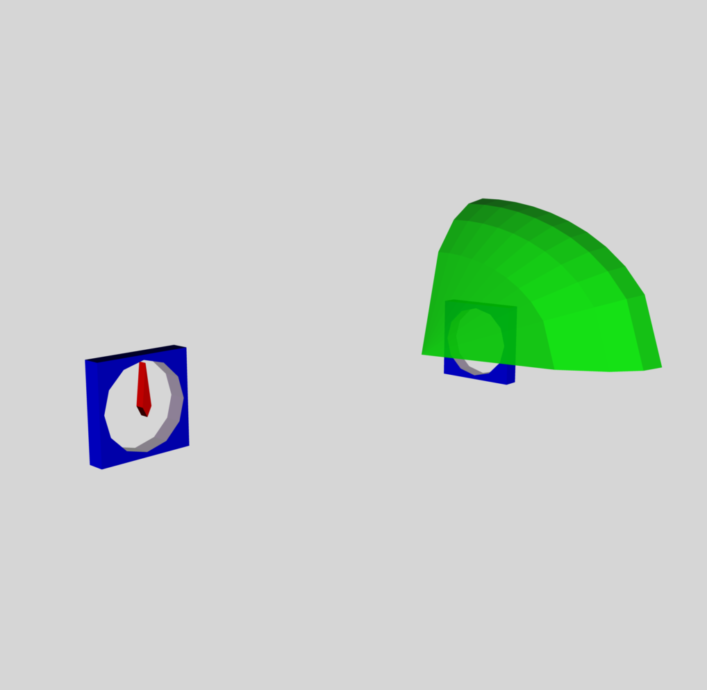
Here, we have added another desirable element to the visual scene, specifically, one octant of the surface of an ellipsoid whose axis ratios are b/a = 0.75 and c/a = 0.50. We generated the data needed to define the relevant vertices and polygons using a home-developed fortran algorithm. This data was printed out from the fortran code in a format that created a new <geometry id="EllipsoidOctant"> subsection for the COLLADA-based xml file; see the Example #9 code presented immediately below.

Example #9A — Building One Octant of an Ellipsoid

<?xml version="1.0" encoding="utf-8"?>
<COLLADA xmlns="http://www.collada.org/2005/11/COLLADASchema" version="1.4.1">
<!--
On 23 September 2019 I copied the following cube-animation file from github:
https://github.com/chinedufn/collada-dae-parser/blob/master/test/fixture/animated-blender-cube.dae
I have made substantial modifications in order to better understand how the animation instructions
actually work.

THIS FILE NAME:  Dropbox/3Dviewers/Clock/Arrow07.PERFECT.dae
It uses "polylist" and correct implementation of "normals" for all polygons of the Clock.
It also displays **two** clocks:  [Initially, we made one spin and the other not.]
It also adds a red "minute hand" to the clock; now, this is the only segment that spins.
-->
  <asset>
    <contributor>
      <author>jet53man</author>
      <authoring_tool>Raw XML</authoring_tool>
    </contributor>
    <created>2019-09-24</created>
    <modified>2019-09-29</modified>
    <unit name="meter" meter="1"/>
    <up_axis>Z_UP</up_axis>
  </asset>
  <library_images/>
    <library_effects>
        <effect id="ID5">
            <profile_COMMON>
                <technique sid="COMMON">
                    <lambert>
                        <diffuse>
                            <color>0 0 1 1</color>
                        </diffuse>
                    </lambert>
                </technique>
            </profile_COMMON>
        </effect>
        <effect id="InnerID5">
            <profile_COMMON>
                <technique sid="COMMON">
                    <lambert>
                        <diffuse>
                            <color>0.4 0.0 0.7 0.4</color>
                        </diffuse>
                    </lambert>
                </technique>
            </profile_COMMON>
        </effect>
        <effect id="ArrowID5">
            <profile_COMMON>
                <technique sid="COMMON">
                    <lambert>
                        <diffuse>
                            <color>1.0 0.0 0.0 1.0</color>
                        </diffuse>
                    </lambert>
                </technique>
            </profile_COMMON>
        </effect>
        <effect id="EllipID5">
            <profile_COMMON>
                <technique sid="COMMON">
                    <lambert>
                        <diffuse>
                            <color>0.0 1.0 0.0 0.9</color>
                        </diffuse>
                    </lambert>
                </technique>
            </profile_COMMON>
        </effect>
    </library_effects>
    <library_materials>
        <material id="ID6" name="material">
            <instance_effect url="#ID5" />
        </material>
        <material id="InnerID6" name="Inner_material">
            <instance_effect url="#InnerID5" />
        </material>
        <material id="ArrowID6" name="Arrow_material">
            <instance_effect url="#ArrowID5" />
        </material>
        <material id="EllipID6" name="Ellip_material">
            <instance_effect url="#EllipID5" />
        </material>
    </library_materials>
    <library_nodes>
        <node id="ID3" name="cube_component">
            <instance_geometry url="#Clock_OuterEdge">
                <bind_material>
                    <technique_common>
                        <instance_material symbol="Material2" target="#ID6">
                            <bind_vertex_input semantic="UVSET0" input_semantic="TEXCOORD" input_set="0" />
                        </instance_material>
                    </technique_common>
                </bind_material>
            </instance_geometry>
            <instance_geometry url="#Clock_InnerEdge">
                <bind_material>
                    <technique_common>
                        <instance_material symbol="Material2" target="#InnerID6">
                            <bind_vertex_input semantic="UVSET0" input_semantic="TEXCOORD" input_set="0" />
                        </instance_material>
                    </technique_common>
                </bind_material>
            </instance_geometry>
        </node>
        <node id="ArrowID3" name="cube_component">
            <instance_geometry url="#Clock_ArrowEdge">
                <bind_material>
                    <technique_common>
                        <instance_material symbol="Material2" target="#ArrowID6">
                            <bind_vertex_input semantic="UVSET0" input_semantic="TEXCOORD" input_set="0" />
                        </instance_material>
                    </technique_common>
                </bind_material>
            </instance_geometry>
        </node>
        <node id="EllipID3" name="ellipsoid_component">
            <instance_geometry url="#EllipsoidOctant">
                <bind_material>
                    <technique_common>
                        <instance_material symbol="Material2" target="#EllipID6">
                            <bind_vertex_input semantic="UVSET0" input_semantic="TEXCOORD" input_set="0" />
                        </instance_material>
                    </technique_common>
                </bind_material>
            </instance_geometry>
        </node>
    </library_nodes>
    <library_geometries>
        <geometry id="Clock_OuterEdge">
            <mesh>
<!--
            **********************************************
            *
            *  Insert first portion of clock's structure
            *
            **********************************************
-->
                <source id="Clock_Positions">
                  <float_array id="Coordinates01" count="123"> 0.0  1.0  0.2 1.0  1.0  0.2 1.0  0.0  0.2 1.0 -1.0  0.2 0.0 -1.0  0.2 -1.0 -1.0  0.2 -1.0  0.0  0.2 -1.0  1.0  0.2 0.0  1.0 -0.2 1.0  1.0 -0.2 1.0  0.0 -0.2 1.0 -1.0 -0.2 0.0 -1.0 -0.2 -1.0 -1.0 -0.2 -1.0  0.0 -0.2 -1.0  1.0 -0.2 0.9  0.0  0.2 0.779423 0.45 0.2 0.45 0.779423 0.2 0.0  0.9  0.2 -0.45 0.779423 0.2 -0.779423 0.45 0.2 -0.9 0.0 0.2 -0.779423 -0.45 0.2 -0.45 -0.779423 0.2 0.0 -0.9 0.2 0.45 -0.779423 0.2 0.779423 -0.45 0.2 -0.9  0.0  -0.2 -0.779423 0.45 -0.2 -0.45 0.779423 -0.2 -0.0  0.9  -0.2 0.45 0.779423 -0.2 0.779423 0.45 -0.2 0.9 0.0 -0.2 0.779423 -0.45 -0.2 0.45 -0.779423 -0.2 -0.0 -0.9 -0.2 -0.45 -0.779423 -0.2 -0.779423 -0.45 -0.2  0.0 0.0 -0.2</float_array>
                  <technique_common>
                    <accessor source="#Coordinates01" count="41" stride="3">
                            <param name="X" type="float" />
                            <param name="Y" type="float" />
                            <param name="Z" type="float" />
                    </accessor>
                  </technique_common>
                </source>
                <source id="Clock_Normals">
                  <float_array id="InnerNormals01" count="18">
 1.0  0.0  0.0
-1.0  0.0  0.0
 0.0  1.0  0.0
 0.0 -1.0  0.0
 0.0  0.0  1.0
 0.0  0.0 -1.0
                  </float_array>
                    <technique_common>
                        <accessor source="#Normals01" count="6" stride="3">
                            <param name="X" type="float" />
                            <param name="Y" type="float" />
                            <param name="Z" type="float" />
                        </accessor>
                    </technique_common>
                </source>
                <vertices id="Clock_Vertices">
                    <input semantic="POSITION" source="#Clock_Positions" />
                </vertices>
                <polylist count="56" material="Material2">
                    <input semantic="VERTEX" source="#Clock_Vertices" offset="0" />
                    <input semantic="NORMAL" source="#Clock_Normals" offset="1" />
<vcount> 3 3 3 3 3  3 3 3 3 3  3 3 3 3 3  3 3 3 3 3  3 3 3 3 3  3 3 3 3 3  3 3 3 3 3  3 3 3 3 3  3 3 3 3 3  3 3 3 3 3  3 3 3 3 3  3</vcount>
<p> 0 2 1 2 8 2  1 2 9 2 8 2  7 2 0 2 15 2  0 2 8 2 15 2 1 0 2 0 9 0  2 0 10 0 9 0  2 0 3 0 10 0  3 0 11 0 10 0 3 3 4 3 11 3  4 3 12 3 11 3  4 3 5 3 12 3  5 3 13 3 12 3 5 1 6 1 13 1  6 1 14 1 13 1  6 1 7 1 14 1  7 1 15 1 14 1 2 4 17 4 16 4  2 4 1 4 17 4  1 4 18 4 17 4  1 4 0 4 18 4  0 4 19 4 18 4 0 4 20 4 19 4  0 4 7 4 20 4  7 4 21 4 20 4  7 4 6 4 21 4  6 4 22 4 21 4 6 4 23 4 22 4  6 4 5 4 23 4  5 4 24 4 23 4  5 4 4 4 24 4  4 4 25 4 24 4 4 4 26 4 25 4  4 4 3 4 26 4  3 4 27 4 26 4  3 4 2 4 27 4  2 4 16 4 27 4 14 5 29 5 28 5  14 5 15 5 29 5  15 5 30 5 29 5  15 5 8 5 30 5  8 5 31 5 30 5 8 5 32 5 31 5  8 5 9 5 32 5  9 5 33 5 32 5  9 5 10 5 33 5  10 5 34 5 33 5 10 5 35 5 34 5  10 5 11 5 35 5  11 5 36 5 35 5  11 5 12 5 36 5  12 5 37 5 36 5 12 5 38 5 37 5  12 5 13 5 38 5  13 5 39 5 38 5  13 5 14 5 39 5  14 5 28 5 39 5 </p>
                </polylist>
            </mesh>
        </geometry>
        <geometry id="Clock_InnerEdge">
            <mesh>
<!--
            **********************************************
            *
            *  Insert second portion of clock's structure
            *
            **********************************************
-->
                <source id="Clock_InnerPositions">
                  <float_array id="InnerCoordinates01" count="123">
0.0  1.0  0.2 1.0  1.0  0.2 1.0  0.0  0.2 1.0 -1.0  0.2 0.0 -1.0  0.2 -1.0 -1.0  0.2 -1.0  0.0  0.2 -1.0  1.0  0.2 0.0  1.0 -0.2 1.0  1.0 -0.2 1.0  0.0 -0.2 1.0 -1.0 -0.2 0.0 -1.0 -0.2 -1.0 -1.0 -0.2 -1.0  0.0 -0.2 -1.0  1.0 -0.2 0.9  0.0  0.2 0.779423 0.45 0.2 0.45 0.779423 0.2 0.0  0.9  0.2 -0.45 0.779423 0.2 -0.779423 0.45 0.2 -0.9 0.0 0.2 -0.779423 -0.45 0.2 -0.45 -0.779423 0.2 0.0 -0.9 0.2 0.45 -0.779423 0.2 0.779423 -0.45 0.2 -0.9  0.0  -0.2 -0.779423 0.45 -0.2 -0.45 0.779423 -0.2 -0.0  0.9  -0.2 0.45 0.779423 -0.2 0.779423 0.45 -0.2 0.9 0.0 -0.2 0.779423 -0.45 -0.2 0.45 -0.779423 -0.2 -0.0 -0.9 -0.2 -0.45 -0.779423 -0.2 -0.779423 -0.45 -0.2  0.0 0.0 -0.2</float_array>
                  <technique_common>
                    <accessor source="#InnerCoordinates01" count="41" stride="3">
                            <param name="X" type="float" />
                            <param name="Y" type="float" />
                            <param name="Z" type="float" />
                    </accessor>
                  </technique_common>
                </source>
                <source id="Clock_InnerNormals">
                  <float_array id="InnerNormals01" count="54">
 1.0  0.0  0.0
-1.0  0.0  0.0
 0.0  1.0  0.0
 0.0 -1.0  0.0
 0.0  0.0  1.0
 0.0  0.0 -1.0
 -0.965926 -0.258819 0.0
 -0.707107 -0.707107 0.0
 -0.258819 -0.965926 0.0
  0.258819 -0.965926 0.0
  0.707107 -0.707107 0.0
  0.965926 -0.258819 0.0
  0.965926  0.258819 0.0
  0.707107  0.707107 0.0
  0.258819  0.965926 0.0
 -0.258819  0.965926 0.0
 -0.707107  0.707107 0.0
 -0.965926  0.258819 0.0
                  </float_array>
                    <technique_common>
                        <accessor source="#InnerNormals01" count="18" stride="3">
                            <param name="X" type="float" />
                            <param name="Y" type="float" />
                            <param name="Z" type="float" />
                        </accessor>
                    </technique_common>
                </source>
                <vertices id="Clock_InnerVertices">
                    <input semantic="POSITION" source="#Clock_InnerPositions" />
                </vertices>
                <polylist count="24" material="Material2">
                    <input semantic="VERTEX" source="#Clock_InnerVertices" offset="0" />
                    <input semantic="NORMAL" source="#Clock_InnerNormals" offset="1"/>
<vcount>4 4 4 4  4 4 4 4  4 4 4 4  3 3 3 3  3 3 3 3  3 3 3 3</vcount>
<p> 16 6 17 6 33 6 34 6 17 7 18 7 32 7 33 7 18 8 19 8 31 8 32 8 19 9 20 9 30 9 31 9 20 10 21 10 29 10 30 10 21 11 22 11 28 11 29 11 22 12 23 12 39 12 28 12 23 13 24 13 38 13 39 13 24 14 25 14 37 14 38 14 25 15 26 15 36 15 37 15 26 16 27 16 35 16 36 16 27 17 16 17 34 17 35 17 28 5 29 5 40 5 29 5 30 5 40 5 30 5 31 5 40 5 31 5 32 5 40 5 32 5 33 5 40 5 33 5 34 5 40 5 34 5 35 5 40 5 35 5 36 5 40 5 36 5 37 5 40 5 37 5 38 5 40 5 38 5 39 5 40 5 39 5 28 5 40 5 </p>
              </polylist>
            </mesh>
        </geometry>
        <geometry id="Clock_ArrowEdge">
            <mesh>
<!--
            **********************************************
            *
            *  Insert arrow portion of clock's structure
            *
            **********************************************
-->
                <source id="Clock_ArrowPositions">
                  <float_array id="ArrowCoordinates01" count="30"> 0.0  0.85 0.25 0.1  0.0 0.25 0.0 -0.2 0.25 -0.1  0.0 0.25 0.0  0.85 0.05 0.1  0.0 0.05 0.0 -0.2 0.05 -0.1  0.0 0.05 0.0  0.0 0.25 0.0  0.0 0.05 </float_array>
                  <technique_common>
                    <accessor source="#ArrowCoordinates01" count="10" stride="3">
                            <param name="X" type="float" />
                            <param name="Y" type="float" />
                            <param name="Z" type="float" />
                    </accessor>
                  </technique_common>
                </source>
                <source id="Clock_ArrowNormals">
                  <float_array id="ArrowNormals01" count="18">
 0  0  1
 0  0 -1
 0.993151  0.116841 0.0
 0.447214 -0.894427 0.0
-0.447214 -0.894427 0.0
-0.993151  0.116841 0.0
                  </float_array>
                    <technique_common>
                        <accessor source="#ArrowNormals01" count="6" stride="3">
                            <param name="X" type="float" />
                            <param name="Y" type="float" />
                            <param name="Z" type="float" />
                        </accessor>
                    </technique_common>
                </source>
                <vertices id="Clock_ArrowVertices">
                    <input semantic="POSITION" source="#Clock_ArrowPositions" />
                </vertices>
                <polylist count="12" material="Material2">
                    <input semantic="VERTEX" source="#Clock_ArrowVertices" offset="0" />
                    <input semantic="NORMAL" source="#Clock_ArrowNormals" offset="1"/>
<vcount>3 3 3 3 3 3 3 3 4 4 4 4</vcount>
<p> 0 0 8 0 1 0 1 0 8 0 2 0 2 0 8 0 3 0 3 0 8 0 0 0 4 1 5 1 9 1 5 1 6 1 9 1 6 1 7 1 9 1 7 1 4 1 9 1 0 2 1 2 5 2 4 2 1 3 2 3 6 3 5 3 2 4 3 4 7 4 6 4 3 5 0 5 4 5 7 5 </p>
              </polylist>
            </mesh>
        </geometry>
<geometry id="EllipsoidOctant">
  <mesh>
<source id="Ellipsoid_Positions">
<float_array id="Ellipsoid_Coordinates" count="135">
    0.0000    0.0000    0.5000
    0.0000    0.7500    0.0000
    0.1000    0.7462    0.0000
    0.2000    0.7348    0.0000
    0.3000    0.7155    0.0000
    0.4000    0.6874    0.0000
    0.5000    0.6495    0.0000
    0.6000    0.6000    0.0000
    0.7000    0.5356    0.0000
    0.8000    0.4500    0.0000
    0.9000    0.3269    0.0000
    1.0000    0.0000    0.0000
    0.0000    0.7262    0.1250
    0.0968    0.7225    0.1250
    0.1936    0.7115    0.1250
    0.2905    0.6927    0.1250
    0.3873    0.6656    0.1250
    0.4841    0.6289    0.1250
    0.5809    0.5809    0.1250
    0.6778    0.5186    0.1250
    0.7746    0.4357    0.1250
    0.8714    0.3165    0.1250
    0.9682    0.0000    0.1250
    0.0000    0.6495    0.2500
    0.0866    0.6463    0.2500
    0.1732    0.6364    0.2500
    0.2598    0.6196    0.2500
    0.3464    0.5953    0.2500
    0.4330    0.5625    0.2500
    0.5196    0.5196    0.2500
    0.6062    0.4638    0.2500
    0.6928    0.3897    0.2500
    0.7794    0.2831    0.2500
    0.8660    0.0000    0.2500
    0.0000    0.4961    0.3750
    0.0661    0.4936    0.3750
    0.1323    0.4861    0.3750
    0.1984    0.4732    0.3750
    0.2646    0.4547    0.3750
    0.3307    0.4296    0.3750
    0.3969    0.3969    0.3750
    0.4630    0.3543    0.3750
    0.5292    0.2976    0.3750
    0.5953    0.2162    0.3750
    0.6614    0.0000    0.3750
</float_array>
<technique_common>
  <accessor source="#Ellipsoid_Coordinates" count="   45" stride="3">
        <param name="X" type="float" />
        <param name="Y" type="float" />
        <param name="Z" type="float" />
  </accessor>
</technique_common>
</source>
<source id="Ellipsoid_Normals">
<float_array id="Ellipsoid_Normals01" count="210">
    0.0092    0.2443    0.9696
    0.0276    0.2419    0.9699
    0.0460    0.2371    0.9704
    0.0644    0.2295    0.9712
    0.0829    0.2190    0.9722
    0.1015    0.2051    0.9735
    0.1203    0.1868    0.9750
    0.1393    0.1627    0.9768
    0.1587    0.1289    0.9789
    0.1854    0.0567    0.9810
    0.0237    0.6314    0.7751
    0.0237    0.6314    0.7751
    0.0713    0.6261    0.7764
    0.0713    0.6261    0.7764
    0.1193    0.6154    0.7792
    0.1193    0.6154    0.7792
    0.1680    0.5985    0.7833
    0.1680    0.5985    0.7833
    0.2176    0.5746    0.7890
    0.2176    0.5746    0.7890
    0.2685    0.5422    0.7962
    0.2685    0.5422    0.7962
    0.3211    0.4987    0.8051
    0.3211    0.4987    0.8051
    0.3760    0.4393    0.8159
    0.3760    0.4393    0.8159
    0.4344    0.3529    0.8287
    0.4344    0.3529    0.8287
    0.5149    0.1575    0.8427
    0.5149    0.1575    0.8427
    0.0320    0.8520    0.5226
    0.0320    0.8520    0.5226
    0.0964    0.8461    0.5242
    0.0964    0.8461    0.5242
    0.1617    0.8340    0.5276
    0.1617    0.8340    0.5276
    0.2287    0.8148    0.5328
    0.2287    0.8148    0.5328
    0.2981    0.7871    0.5400
    0.2981    0.7871    0.5400
    0.3708    0.7488    0.5493
    0.3708    0.7488    0.5493
    0.4481    0.6958    0.5613
    0.4481    0.6958    0.5613
    0.5315    0.6209    0.5762
    0.5315    0.6209    0.5762
    0.6239    0.5069    0.5947
    0.6239    0.5069    0.5947
    0.7533    0.2304    0.6160
    0.7533    0.2304    0.6160
    0.0369    0.9817    0.1870
    0.0369    0.9817    0.1870
    0.1112    0.9759    0.1878
    0.1112    0.9759    0.1878
    0.1869    0.9639    0.1894
    0.1869    0.9639    0.1894
    0.2652    0.9449    0.1919
    0.2652    0.9449    0.1919
    0.3473    0.9172    0.1954
    0.3473    0.9172    0.1954
    0.4348    0.8780    0.2001
    0.4348    0.8780    0.2001
    0.5298    0.8227    0.2061
    0.5298    0.8227    0.2061
    0.6353    0.7421    0.2139
    0.6353    0.7421    0.2139
    0.7564    0.6146    0.2240
    0.7564    0.6146    0.2240
    0.9292    0.2842    0.2361
    0.9292    0.2842    0.2361
</float_array>
<technique_common>
  <accessor source="#Ellipsoid_Normals01" count="   70" stride="3">
        <param name="X" type="float" />
        <param name="Y" type="float" />
        <param name="Z" type="float" />
  </accessor>
</technique_common>
</source>
<vertices id="Ellipsoid_Vertices">
  <input semantic="POSITION" source="#Ellipsoid_Positions" />
</vertices>
<polylist count="   70" material="Material2">
  <input semantic="VERTEX" source="#Ellipsoid_Vertices" offset="0" />
  <input semantic="NORMAL" source="#Ellipsoid_Normals" offset="1" />
<vcount> 3 3 3 3 3  3 3 3 3 3  3 3 3 3 3  3 3 3 3 3  3 3 3 3 3  3 3 3 3 3  3 3 3 3 3  3 3 3 3 3  3 3 3 3 3  3 3 3 3 3  3 3 3 3 3  3 3 3 3 3  3 3 3 3 3  3 3 3 3 3  </vcount>
<p>
    0    0   35    0   34    0
    0    1   36    1   35    1
    0    2   37    2   36    2
    0    3   38    3   37    3
    0    4   39    4   38    4
    0    5   40    5   39    5
    0    6   41    6   40    6
    0    7   42    7   41    7
    0    8   43    8   42    8
    0    9   44    9   43    9
   34   10   24   10   23   10
   34   11   35   11   24   11
   35   12   25   12   24   12
   35   13   36   13   25   13
   36   14   26   14   25   14
   36   15   37   15   26   15
   37   16   27   16   26   16
   37   17   38   17   27   17
   38   18   28   18   27   18
   38   19   39   19   28   19
   39   20   29   20   28   20
   39   21   40   21   29   21
   40   22   30   22   29   22
   40   23   41   23   30   23
   41   24   31   24   30   24
   41   25   42   25   31   25
   42   26   32   26   31   26
   42   27   43   27   32   27
   43   28   33   28   32   28
   43   29   44   29   33   29
   23   30   13   30   12   30
   23   31   24   31   13   31
   24   32   14   32   13   32
   24   33   25   33   14   33
   25   34   15   34   14   34
   25   35   26   35   15   35
   26   36   16   36   15   36
   26   37   27   37   16   37
   27   38   17   38   16   38
   27   39   28   39   17   39
   28   40   18   40   17   40
   28   41   29   41   18   41
   29   42   19   42   18   42
   29   43   30   43   19   43
   30   44   20   44   19   44
   30   45   31   45   20   45
   31   46   21   46   20   46
   31   47   32   47   21   47
   32   48   22   48   21   48
   32   49   33   49   22   49
   12   50    2   50    1   50
   12   51   13   51    2   51
   13   52    3   52    2   52
   13   53   14   53    3   53
   14   54    4   54    3   54
   14   55   15   55    4   55
   15   56    5   56    4   56
   15   57   16   57    5   57
   16   58    6   58    5   58
   16   59   17   59    6   59
   17   60    7   60    6   60
   17   61   18   61    7   61
   18   62    8   62    7   62
   18   63   19   63    8   63
   19   64    9   64    8   64
   19   65   20   65    9   65
   20   66   10   66    9   66
   20   67   21   67   10   67
   21   68   11   68   10   68
   21   69   22   69   11   69
</p>
</polylist>
  </mesh>
</geometry>
    </library_geometries>
  <library_animations>
    <animation id="Cube_rotation_euler_Z">
      <source id="Cube_rotation_euler_Z-input">
<!--        <float_array id="Cube_rotation_euler_Z-input-array" count="5">0 0.2083333 0.4166666 0.625 0.8333333</float_array> -->
<!--        <float_array id="Cube_rotation_euler_Z-input-array" count="5">0 0.4167 0.8333 1.25 1.666</float_array> -->
        <float_array id="Cube_rotation_euler_Z-input-array" count="17">0 0.25 0.5 0.75 1.0 1.25 1.5 1.75 2.0 2.25 2.5 2.75 3.0 3.25 3.5 3.75 4.0</float_array>
        <technique_common>
          <accessor source="#Cube_rotation_euler_Z-input-array" count="5" stride="1">
            <param name="TIME" type="float"/>
          </accessor>
        </technique_common>
      </source>
      <source id="Cube_rotation_euler_Z-output">
<!--        <float_array id="Cube_rotation_euler_Z-output-array" count="5">0 -22.5 -45 -67.5 -90</float_array> -->
        <float_array id="Cube_rotation_euler_Z-output-array" count="17">0 -22.5 -45 -67.5 -90 -112.5 -135.0 -157.5 -180.0 -202.5 -225.0 -247.5 -270.0 -292.5 -315.0 -337.5 -360.0</float_array>
        <technique_common>
          <accessor source="#Cube_rotation_euler_Z-output-array" count="5" stride="1">
            <param name="ANGLE" type="float"/>
          </accessor>
        </technique_common>
      </source>
      <sampler id="Cube_rotation_euler_Z-sampler">
        <input semantic="INPUT" source="#Cube_rotation_euler_Z-input"/>
        <input semantic="OUTPUT" source="#Cube_rotation_euler_Z-output"/>
      </sampler>
      <channel source="#Cube_rotation_euler_Z-sampler" target="jetman/rotationZ.ANGLE"/>
    </animation>
    <animation id="Cube_scale_Z">
      <source id="Cube_scale_Z-input">
<!--        <float_array id="Cube_scale_Z-input-array" count="5">0 0.2083333 0.4166666 0.625 0.8333333</float_array>  -->
        <float_array id="Cube_scale_Z-input-array" count="5">0 0.0694 0.1389 0.2083 0.2778</float_array>
        <technique_common>
          <accessor source="#Cube_scale_Z-input-array" count="5" stride="1">
            <param name="TIME" type="float"/>
          </accessor>
        </technique_common>
      </source>
      <source id="Cube_scale_Z-output">
<!--    <float_array id="Cube_scale_Z-output-array" count="5">0.5 0.4 0.3 0.2 0.1</float_array>  -->
        <float_array id="Cube_scale_Z-output-array" count="5">1.0 1.0 1.0 1.0 1.0</float_array>
        <technique_common>
          <accessor source="#Cube_scale_Z-output-array" count="5" stride="1">
            <param name="Z" type="float"/>
          </accessor>
        </technique_common>
      </source>
      <sampler id="Cube_scale_Z-sampler">
        <input semantic="INPUT" source="#Cube_scale_Z-input"/>
        <input semantic="OUTPUT" source="#Cube_scale_Z-output"/>
      </sampler>
      <channel source="#Cube_scale_Z-sampler" target="jetman/scale.Z"/>
    </animation>
  </library_animations>
    <library_controllers/>
    <library_visual_scenes>
        <visual_scene id="EntireLayout">
<!--
***********
*
* Evidently, it is important for the "id" of this node to be shared
* with the "directory" name that is used in the animation "channel"
* instructions.  For example, "jetman" is used here.
*
***********
-->
          <node id="TwoClocks">
            <node id="firstclock" name="instance_1">
              <translate>0.0 1.0 0.0</translate>
              <rotate sid="rotationX">1 0 0 90</rotate>
              <rotate sid="rotationZ">0 0 1 0</rotate>
<!--
              <rotate sid="rotationY">0 1 0 90</rotate>
-->
              <scale sid="scale">1 1 1</scale>
              <instance_node url="#ID3" />
            </node>
            <node id="jetman" name="instance_Arrow">
              <translate>0.0 1.0 0.0</translate>
              <rotate sid="rotationX">1 0 0 90</rotate>
              <rotate sid="rotationZ">0 0 1 0</rotate>
<!--
              <rotate sid="rotationY">0 1 0 90</rotate>
-->
              <scale sid="scale">1 1 1</scale>
              <instance_node url="#ArrowID3" />
            </node>
            <extra>
              <technique profile="FCOLLADA">
                <start_time>0</start_time>
                <end_time>4.0</end_time>
              </technique>
            </extra>
            <node id="secondClock" name="instance_2">
              <translate>10.0 0.0 0.0</translate>
<!--
              <rotate sid="rotationZ">0 0 1 90</rotate>
-->
              <rotate sid="rotationX">1 0 0 90</rotate>
              <rotate sid="rotationY">0 1 0 -90</rotate>
              <scale sid="scale">1 1 1</scale>
              <instance_node url="#ID3" />
            </node>
            <node id="EllipScene" name="instance_Ellip">
              <translate>10.0 0.0 0.0</translate>
<!--
              <rotate sid="rotationZ">0 0 1 90</rotate>
-->
              <rotate sid="rotationX">1 0 0 90</rotate>
              <rotate sid="rotationY">0 1 0 -90</rotate>
              <scale sid="scale">5.0 5.0 5.0</scale>
              <instance_node url="#EllipID3" />
            </node>
          </node>
        </visual_scene>
    </library_visual_scenes>
    <scene>
        <instance_visual_scene url="#EntireLayout" />
    </scene>
</COLLADA>

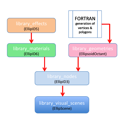
Here we document the various lines of the COLLADA-based <xml> code that require a unique new "id" tag when a new geometry node is added:

<library_effects>

<effect id="EllipID5">

<library_materials>

<material id="EllipID6" name="Ellip_material">
<instance_effect url="#EllipID5" />

<library_nodes>

<node id="EllipID3" name="ellipsoid_component">
<instance_geometry url="#EllipsoidOctant">
<instance_material symbol="Material2" target="#EllipID6">

<library_geometries> — this group provided by fortran output

<geometry id="EllipsoidOctant">
<source id="Ellipsoid_Positions">
<float_array id="Ellipsoid_Coordinates" count="135">
<accessor source="#Ellipsoid_Coordinates" count=" 45" stride="3">
<source id="Ellipsoid_Normals">
<float_array id="Ellipsoid_Normals01" count="210">
<accessor source="#Ellipsoid_Normals01" count=" 70" stride="3">
<vertices id="Ellipsoid_Vertices">
<input semantic="POSITION" source="#Ellipsoid_Positions" />
<polylist count=" 70" material="Material2">
<input semantic="VERTEX" source="#Ellipsoid_Vertices" offset="0" />
<input semantic="NORMAL" source="#Ellipsoid_Normals" offset="1" />

<library_visual_scenes>

<node id="EllipScene" name="instance_Ellip">
<instance_node url="#EllipID3" />

Example #9B — FORTRAN code that Generated Vertices & Polygons

      Program ThreeDEllipsoids
!!!!!!!!
!
!  Surface of one Octant of the Ellipsoid
!
!!!!!!!!
!          
      real*8 bovera,covera
      real*8 zlayer(5),xvalue(4,11),yvalue
      real*8 pt3xx(200),pt3yy(200),pt3zz(200)
      real*8 xmax,dx
      real*8 x1,y1,z1,x2,y2,z2,x3,y3,z3,xnorm,ynorm,znorm
      integer n,nzmax,m,mxmax,ncount,npt
      integer ell,nverts,numtri,nt1,nt2,nfloats
      integer ellmin,ellmax,nzslice
      integer triangle(200,4)
  501 format(8x,'pt num',6x,'x',10x,'y',10x,'z',/)
  502 format(I10,3F15.7)
  503 format(//,5x,'nverts = ',I5,/)
  504 format(/,6x,'Triangle No.',3x,'Vertex1',3x,'Vertex2',3x,'Vertex3')
  505 format(I10,5x,3I10,5x,3f13.5)
  507 format(//,5x,'numtri = ',I5,/)
  510 format(/,'nzslice, numtri, ellmin, ellmax = ',4I8)
  599 format('<geometry id="EllipsoidOctant">')
  600 format(2x,'<mesh>')
  601 format('<source id="Ellipsoid_Positions">',/,'<float_array id="Ellipsoid_Coordinates" count="',I3,'">'/)
  602 format(3F10.4)
  603 format('</float_array>')
  604 format('<technique_common>')
  605 format(2x,'<accessor source="#Ellipsoid_Coordinates" count="',I5,&
     &'" stride="3">')
  606 format(8x,'<param name="X" type="float" />')
  607 format(8x,'<param name="Y" type="float" />')
  608 format(8x,'<param name="Z" type="float" />')
  609 format(2x,'</accessor>',/,'</technique_common>',/,'</source>')
  610 format('<source id="Ellipsoid_Normals">',/,'<float_array id="Ellipsoid_Normals01" count="',I3,'">'/)
  611 format(2x,'<accessor source="#Ellipsoid_Normals01" count="',I5,&
     &'" stride="3">')
  612 format('<vertices id="Ellipsoid_Vertices">')
  613 format(2x,'<input semantic="POSITION"',&
     &' source="#Ellipsoid_Positions" />')
  614 format('</vertices>')
  615 format('<polylist count="',I5,'" material="Material2">')
  616 format(2x,'<input semantic="VERTEX"',&
     &' source="#Ellipsoid_Vertices" offset="0" />')
  617 format(2x,'<input semantic="NORMAL"',&
     &' source="#Ellipsoid_Normals" offset="1" />',/,'<vcount></vcount>',/,'<p>')
  618 format('</p>',/,'</polylist>')
  619 format(2x,'</mesh>')
  620 format('</geometry>')
  621 format(6I5)
! zlayer is z/a; its vector length is (nzmax+1). 
! xvalue is x/a; its array lengths are (nzmax,mxmax+1).
! yvalue is y/a.
      bovera = 0.75d0
      covera = 0.50d0
      nzmax  = 4
      mxmax  = 10
      zlayer(nzmax+1) = covera
      pt3xx(1) = 0.0d0
      pt3yy(1) = 0.0d0
      pt3zz(1) = zlayer(nzmax+1)
      ncount  = 1
      do n = 1,nzmax
        zlayer(n) = covera*dfloat((n-1))/dfloat(nzmax)
        xmax = dsqrt(1.0d0 - (zlayer(n)/covera)**2)
        dx   = xmax/dfloat(mxmax)
        do m = 1,mxmax+1
          xvalue(n,m) = dfloat(m-1)*dx
            ncount = ncount+1            
            if(m.eq.(mxmax+1))then
            yvalue = 0.0d0
            else
            yvalue = bovera*dsqrt(1.0d0 - (zlayer(n)/covera)**2 - xvalue(n,m)**2)
            endif
            pt3xx(ncount) = xvalue(n,m)
            pt3yy(ncount) = yvalue
            pt3zz(ncount) = zlayer(n)
        enddo
      enddo
      nverts = ncount
      nfloats = 3*nverts
!     write(*,503)nverts
      write(*,599)
      write(*,600)
      write(*,601)nfloats
!     write(*,501)
!     do n=1,ncount
!     npt = n - 1
!     write(*,502)npt,pt3xx(n),pt3yy(n),pt3zz(n)
!     enddo
      do n=1,ncount
      write(*,602)pt3xx(n),pt3yy(n),pt3zz(n)
      enddo
      write(*,603)
      write(*,604)
      write(*,605)nverts
!!!
!!!   Finished determining coordinates of all [nzmax x (mxmax+1) + 1] vertices.
!!!
!!!   Now identify triangles
!     write(*,504)
      nt1 = 0
      nt2 = nverts - mxmax
      numtri = 0
      do ell=1,mxmax
      triangle(ell,1) = nt1
      triangle(ell,2) = nt2-1
      triangle(ell,3) = nt2
      triangle(ell,4) = ell-1
      nt2 = nt2 + 1
!     write(*,505)triangle(numtri+1,4),triangle(numtri+1,1),&
!    &triangle(numtri+1,2),triangle(numtri+1,3)
      numtri = numtri+1
      enddo
        numtri = numtri+1
      do nzslice=1,nzmax-1
!!!!!
!
!   Phase 2
!
!!!!!
!     nzslice=1
        ellmin = nverts - nzslice*(mxmax+1)
        ellmax = ellmin + mxmax - 1
!       numtri = numtri+1
!       write(*,510)nzslice,numtri,ellmin,ellmax
        do ell=ellmin,ellmax
        triangle(numtri,1) = ell
        triangle(numtri,2) = ell-(mxmax+1)
        triangle(numtri,3) = ell - mxmax
        triangle(numtri,4) = numtri-1
          numtri = numtri + 1
        triangle(numtri,1) = ell 
        triangle(numtri,2) = ell - mxmax
        triangle(numtri,3) = ell + 1
        triangle(numtri,4) = numtri-1
          numtri = numtri + 1
        enddo
      enddo
      numtri = numtri-1
!!!!!
!
!     write(*,507)numtri
!
!!!!!
      nfloats=3*numtri
      write(*,606)
      write(*,607)
      write(*,608)
      write(*,609)
      write(*,610)nfloats
      do nt1=1,numtri
      n1st = triangle(nt1,1)
      n2nd = triangle(nt1,2)
      n3rd = triangle(nt1,3)
      x1 = pt3xx(n1st+1)
      y1 = pt3yy(n1st+1)
      z1 = pt3zz(n1st+1)
      x2 = pt3xx(n2nd+1)
      y2 = pt3yy(n2nd+1)
      z2 = pt3zz(n2nd+1)
      x3 = pt3xx(n3rd+1)
      y3 = pt3yy(n3rd+1)
      z3 = pt3zz(n3rd+1)
      call Normals(x1,y1,z1,x2,y2,z2,x3,y3,z3,xnorm,ynorm,znorm)
!     write(*,505)triangle(nt1,4),triangle(nt1,1),&
!    &triangle(nt1,2),triangle(nt1,3),xnorm,ynorm,znorm
      write(*,602)xnorm,ynorm,znorm
      enddo
      write(*,603)
      write(*,604)
      write(*,611)numtri
      write(*,606)
      write(*,607)
      write(*,608)
      write(*,609)
      write(*,612)
      write(*,613)
      write(*,614)
      write(*,615)numtri
      write(*,616)
      write(*,617)
!
      do nt1=1,numtri
        write(*,621)triangle(nt1,1),triangle(nt1,4),&
     &              triangle(nt1,3),triangle(nt1,4),&
     &              triangle(nt1,2),triangle(nt1,4)
      enddo
!
      write(*,618)
      write(*,619)
      write(*,620)
      stop
      end program ThreeDEllipsoids
      Subroutine Normals(x1,y1,z1,x2,y2,z2,x3,y3,z3,xnorm,ynorm,znorm)
      real*8 x1,y1,z1,x2,y2,z2,x3,y3,z3,xnorm,ynorm,znorm
      real*8 xlength,ylength,zlength,length
      xlength = (y2-y1)*(z3-z1) - (y3-y1)*(z2-z1)
      ylength = (z2-z1)*(x3-x1) - (z3-z1)*(x2-x1)
      zlength = (x2-x1)*(y3-y1) - (x3-x1)*(y2-y1)
      length  = dsqrt(xlength**2 + ylength**2 + zlength**2)
      xnorm   = -xlength/length
      ynorm   = -ylength/length
      znorm   = -zlength/length
      return
      end

In the fortran code, "Subroutine Normals" is called upon to determine the normal (unit vector) to the plane that is uniquely defined by each individual triangle. It accomplishes this as follows. The vectors that extend from the coordinate origin to, respectively, the 1^st, 2^nd and 3^rd vertex of the relevant triangle are defined by the expressions,

<math>~{\vec{x}}_1</math>	<math>~=</math>	<math>~\hat{i}x_1 + \hat{j} y_1 + \hat{k} z_1 \, ,</math>
<math>~{\vec{x}}_2</math>	<math>~=</math>	<math>~\hat{i}x_2 + \hat{j} y_2 + \hat{k} z_2 \, ,</math>
<math>~{\vec{x}}_3</math>	<math>~=</math>	<math>~\hat{i}x_3 + \hat{j} y_3 + \hat{k} z_3 \, .</math>

The vector that points from the first vertex — associated with coordinate point <math>~(x_1, y_1, z_1)</math> — to the second vertex — associated with coordinate point <math>~(x_2, y_2, z_2)</math> — is,

@@ Line 3,277: / Line 3,277: @@
 </td>
 </tr></table>
+In the fortran code, "Subroutine Normals" is called upon to determine the normal (unit vector) to the plane that is uniquely defined by each individual triangle.  It accomplishes this as follows.  The vectors that extend from the coordinate origin to, respectively, the 1<sup>st</sup>, 2<sup>nd</sup> and 3<sup>rd</sup> vertex of the relevant triangle are defined by the expressions,
+<table border="0" cellpadding="5" align="center">
+<tr>
+  <td align="right">
+<math>~{\vec{x}}_1</math>
+  </td>
+  <td align="center">
+<math>~=</math>
+  </td>
+  <td align="left">
+<math>~\hat{i}x_1 + \hat{j} y_1 + \hat{k} z_1 \, ,</math>
+  </td>
+</tr>
+<tr>
+  <td align="right">
+<math>~{\vec{x}}_2</math>
+  </td>
+  <td align="center">
+<math>~=</math>
+  </td>
+  <td align="left">
+<math>~\hat{i}x_2 + \hat{j} y_2 + \hat{k} z_2 \, ,</math>
+  </td>
+</tr>
+<tr>
+  <td align="right">
+<math>~{\vec{x}}_3</math>
+  </td>
+  <td align="center">
+<math>~=</math>
+  </td>
+  <td align="left">
+<math>~\hat{i}x_3 + \hat{j} y_3 + \hat{k} z_3 \, .</math>
+  </td>
+</tr>
+</table>
+The vector that points from the first vertex &#8212; associated with coordinate point <math>~(x_1, y_1, z_1)</math> &#8212; to the second vertex  &#8212; associated with coordinate point <math>~(x_2, y_2, z_2)</math> &#8212; is,
+<table border="0" cellpadding="5" align="center">
+<tr>
+  <td align="right">
+<math>~{\vec{x}}_{12}</math>
+  </td>
+  <td align="center">
+<math>~=</math>
+  </td>
+  <td align="left">
+<math>~{\vec{x}}_2 - {\vec{x}}_1</math>
+  </td>
+  <td align="center">
+<math>~=</math>
+  </td>
+  <td align="center">
+<math>~\hat{i}(x_2 - x_1) + \hat{j}(y_2 - y_1) _ \hat{k}(z_2 - z_1) \, ;</math>
+  </td>
+</tr>
+</table>
 {{LSU_HBook_footer}}

Difference between revisions of "User:Tohline/Appendix/Ramblings/VirtualReality"