Difference between revisions of "User:Tohline/ThreeDimensionalConfigurations/JacobiEllipsoids"
(→Roots of the Governing Relation: More captions to three segments of Table !) |
(→Roots of the Governing Relation: Explain Tables 1 and 2 after moving the "old" Segment A to a different chapter) |
||
| Line 489: | Line 489: | ||
</th> | </th> | ||
</tr> | </tr> | ||
<tr><td align="left"> | <tr><td align="left"> | ||
<pre> | <pre> | ||
| Line 562: | Line 520: | ||
</pre> | </pre> | ||
</td></tr> | </td></tr> | ||
< | </table> | ||
<b>Table | |||
</ | <b>With regard to our Table 1 (immediately above):</b> Given each pair of axis ratios, <math>~(\tfrac{b}{a},\tfrac{c}{a})</math> — copied from Table IV of EFE (see columns 1 and 2 of our Table 1) — and the corresponding coefficient values, <math>~A_1</math>, <math>~A_2</math>, and <math>~A_3</math>, as tabulated in [[User:Tohline/ThreeDimensionalConfigurations/HomogeneousEllipsoids#Table2|Table 2 of our accompanying discussion]], we calculated corresponding values of <math>~\Omega^2</math> (column 3) and total angular momentum (column 4) in the units used in EFE's Table IV, as well as (column 5) the total angular momentum in units used by [http://adsabs.harvard.edu/abs/1995ApJ...446..472C Christodoulou, ''et al.'' (1995, ApJ, 446, 472)] — see [[User:Tohline/ThreeDimensionalConfigurations/HomogeneousEllipsoids#Example_Evaluations|our related discussion of these physical quantities]]. We also have tabulated associated values of the function, <math>~f_J</math>, (column 6) and its first derivative, <math>~f_J^'</math>, (column 7) as defined immediately above. Notice that <math>~f_J</math> is very nearly zero in all cases, which indicates that each axis-ratio pair indeed identifies a configuration that lies along the Jacobi sequence. | ||
<table border="1" cellpadding="5" align="center"> | |||
<tr> | |||
<th align="center" colspan="1"> | |||
<font size="+1">Table 2: Jacobi Sequence</font> | |||
</th> | |||
</tr> | |||
<tr><td align="left"> | <tr><td align="left"> | ||
<pre> | <pre> | ||
| Line 593: | Line 558: | ||
</td></tr> | </td></tr> | ||
</table> | </table> | ||
<b>With regard to our Table 2 (immediately above):</b> Here we specified twenty-one values of the axis ratio, <math>~\tfrac{c}{a}</math>, (column 2) and used our Newton-Raphson-based root finder to identify corresponding values of the companion axis ratio, <math>~\tfrac{b}{a}</math>, (column 1) that satisfies the governing relation, <math>~f_J = 0</math>. | |||
==Sequence Plots== | ==Sequence Plots== | ||
Revision as of 22:36, 26 June 2016

|
|---|
| | Tiled Menu | Tables of Content | Banner Video | Tohline Home Page | |
Jacobi Ellipsoids
General Coefficient Expressions
As has been detailed in an accompanying chapter, the gravitational potential anywhere inside or on the surface, <math>~(a_1,a_2,a_3) ~\leftrightarrow~(a,b,c)</math>, of an homogeneous ellipsoid may be given analytically in terms of the following three coefficient expressions:
|
<math> ~A_1 </math> |
<math> ~= </math> |
<math>~2\biggl(\frac{b}{a}\biggr)\biggl(\frac{c}{a}\biggr) \biggl[ \frac{F(\theta,k) - E(\theta,k)}{k^2 \sin^3\theta} \biggr] \, , </math> |
|
<math> ~A_3 </math> |
<math> ~= </math> |
<math> ~2\biggl(\frac{b}{a}\biggr) \biggl[ \frac{(b/a) \sin\theta - (c/a)E(\theta,k)}{(1-k^2) \sin^3\theta} \biggr] \, , </math> |
|
<math> ~A_2 </math> |
<math> ~= </math> |
<math>~2 - (A_1+A_3) \, ,</math> |
where, <math>~F(\theta,k)</math> and <math>~E(\theta,k)</math> are incomplete elliptic integrals of the first and second kind, respectively, with arguments,
|
<math>~\theta = \cos^{-1} \biggl(\frac{c}{a} \biggr)</math> |
and |
<math>~k = \biggl[\frac{1 - (b/a)^2}{1 - (c/a)^2} \biggr]^{1/2} \, .</math> |
| [ EFE, Chapter 3, §17, Eq. (32) ] | ||
Equilibrium Conditions for Jacobi Ellipsoids
Pulling from Chapter 6 — specifically, §39 — of Chandrasekhar's EFE, we understand that the semi-axis ratios, <math>~(\tfrac{b}{a},\tfrac{c}{a})</math> associated with Jacobi ellipsoids are given by the roots of the equation,
|
<math>~a^2 b^2 A_{12}</math> |
<math>~=</math> |
<math>~c^2 A_3 \, ,</math> |
| [ EFE, §39, Eq. (4) ] | ||
and the associated value of the square of the equilibrium configuration's angular velocity is,
|
<math>~\frac{\Omega^2}{\pi G \rho}</math> |
<math>~=</math> |
<math>~2B_{12} \, ,</math> |
| [ EFE, §39, Eq. (5) ] | ||
where,
|
<math>~A_{12}</math> |
<math>~\equiv</math> |
<math>~-\frac{A_1-A_2}{(a^2 - b^2)} \, ,</math> |
| [ EFE, §21, Eq. (107) ] | ||
|
<math>~B_{12}</math> |
<math>~\equiv</math> |
<math>~A_2 - a^2A_{12} \, .</math> |
| [ EFE, §21, Eq. (105) ] | ||
Taken together, we see that, written in terms of the two primary coefficients, <math>~A_1</math> and <math>~A_3</math>, the pair of defining relations for Jacobi ellipsoids is:
| |||||||||
Roots of the Governing Relation
To simplify notation, here we will set,
|
<math>~x \equiv \frac{b}{a}</math> |
and |
<math>~y \equiv \frac{c}{a} \, ,</math> |
in which case the governing relation is,
|
<math>~f_J</math> |
<math>~=</math> |
<math>~\frac{x^2}{1-x^2} \biggl[ 2(1-A_1)-A_3\biggr]-y^2 A_3 =0 \, .</math> |
Our plan is to employ the Newton-Raphson method to find the root(s) of the <math>~f_J = 0</math> relation, typically holding <math>~y</math> fixed and using the Newton-Raphson technique to identify the corresponding "root" value of <math>~x</math>. Using this approach, the Newton-Raphson technique requires specification of, not only the function, <math>~f_J</math>, but also its first derivative,
|
<math>~f_J^'</math> |
<math>~=</math> |
<math>~\frac{df_J}{dx} \, .</math> |
Let's determine the requisite expression, using a prime superscript to indicate differentiation with respect to <math>~x</math>.
|
<math>~f_J^'</math> |
<math>~=</math> |
<math>~ \biggl[ 2(1-A_1)-A_3\biggr]\biggl[ \frac{2x}{(1-x^2)^2} \biggr] -\frac{x^2}{1-x^2} \biggl[ 2A_1^'+A_3^'\biggr] -y^2 A_3^' \, , </math> |
where, given that <math>~\theta</math> does not depend on <math>~x</math>,
|
<math> ~A_1^' </math> |
<math> ~= </math> |
<math>~\frac{2y}{\sin^3\theta} \cdot \frac{d}{dx}\biggl\{ \frac{x}{k^2} \biggl[ F(\theta,k) - E(\theta,k) \biggr] \biggr\} </math> |
|
|
<math> ~= </math> |
<math>~\frac{2y}{k^3 \sin^3\theta} \cdot \biggl\{ [ F - E ] [k - 2xk^' ] +xk [ F^' - E^' ]\biggr\} \, , </math> |
|
<math> ~A_3^' </math> |
<math> ~= </math> |
<math> ~\frac{2}{\sin^3\theta} \cdot \frac{d}{dx}\biggl\{ \frac{x}{(1-k^2)} \biggl[ x \sin\theta - yE(\theta,k)\biggr] \biggr\} </math> |
|
|
<math> ~= </math> |
<math> ~\frac{2}{(1-k^2)^2\sin^3\theta} \biggl\{ \biggl[ x \sin\theta - yE\biggr]\biggl[ (1-k^2) +2xkk^' \biggr] + x(1-k^2) \biggl[ \sin\theta - yE^'\biggr] \biggr\}\, , </math> |
|
<math>~k^'</math> |
<math>~=</math> |
<math>~ \frac{d}{dx}\biggl[\frac{1 - x^2}{1 - y^2} \biggr]^{1/2} = \frac{-x}{(1 - x^2)^{1/2}(1 - y^2)^{1/2}} \, , </math> |
|
<math>~F^'</math> |
<math>~=</math> |
<math>~ \frac{\partial F(\theta,k)}{\partial k} \cdot k^' \, , </math> |
|
<math>~E^'</math> |
<math>~=</math> |
<math>~ \frac{\partial E(\theta,k)}{\partial k} \cdot k^' \, . </math> |
Now, according to online WolframResearch documentation — see, in particular, the subsection titled, "Representations of Derivatives" —
|
<math>~\frac{\partial F(z|m)}{\partial m}</math> |
<math>~=</math> |
<math>~ \frac{E(z|m)}{2(1-m)m} - \frac{F(z|m)}{2m} - \frac{\sin(2z)}{4(1-m)\sqrt{1-m\sin^2(z)}} \, , </math> |
and,
|
<math>~\frac{\partial E(z|m)}{\partial m}</math> |
<math>~=</math> |
<math>~\frac{E(z|m) - F(z|m)}{2m} \, ,</math> |
where, <math>~z~\leftrightarrow~\theta</math>, and,
<math>~m \equiv k^2 ~~~~\Rightarrow~~~~\frac{dm}{dk} = 2k \ .</math>
Hence, we have,
|
<math>~F^'</math> |
<math>~=</math> |
<math>~ \biggl[\frac{\partial F(z|m)}{\partial m} \cdot \frac{dm}{dk}\biggr] k^' </math> |
|
|
<math>~=</math> |
<math>~ \biggl[ \frac{E(\theta,k)}{2(1-k^2)k^2} - \frac{F(\theta,k)}{2k^2} - \frac{\sin(2\theta)}{4(1-k^2)\sqrt{1-k^2\sin^2\theta}} \biggr] 2kk^' \, , </math> |
|
<math>~E^'</math> |
<math>~=</math> |
<math>~ \biggl[ \frac{\partial E(z|m)}{\partial m} \cdot \frac{dm}{dk}\biggr] k^' </math> |
|
|
<math>~=</math> |
<math>~ \biggl[ E(\theta,k) - F(\theta,k) \biggr] \frac{k^'}{k} \, . </math> |
This, then, gives us all of the expressions necessary to specify the derivative, <math>~f_J^'</math> analytically.
|
Table 1: Double-Precision Evaluations
Related to Table IV in EFE, Chapter 6, §39 (p. 103) |
|---|
         b/a      c/a            omega2              angmom              5L/M                fJ              fJderiv

        1.00   0.582724     3.742297785D-01     3.037510987D-01     4.232965627D+00     0.000000000D+00     0.000000000D+00
        0.96   0.570801     3.739782202D-01     3.039551227D-01     4.235808832D+00     1.377942479D-06     1.636908401D-01
        0.92   0.558330     3.731876801D-01     3.046006837D-01     4.244805137D+00    -6.821687132D-07     1.676406830D-01
        0.88   0.545263     3.717835971D-01     3.057488283D-01     4.260805266D+00     8.533280272D-07     1.715558312D-01
        0.84   0.531574     3.696959199D-01     3.074667323D-01     4.284745355D+00    -4.622993727D-08     1.754024874D-01
        0.80   0.517216     3.668370069D-01     3.098368632D-01     4.317774645D+00     2.805300664D-08     1.791408327D-01
        0.76   0.502147     3.631138118D-01     3.129555079D-01     4.361234951D+00     3.221800126D-07     1.827219476D-01
        0.72   0.486322     3.584232032D-01     3.169377270D-01     4.416729718D+00     3.274773094D-08     1.860866255D-01
        0.68   0.469689     3.526490289D-01     3.219229588D-01     4.486202108D+00     1.202999164D-08     1.891636215D-01
        0.64   0.452194     3.456641138D-01     3.280805511D-01     4.572012092D+00     2.681560312D-07     1.918668912D-01
        0.60   0.433781     3.373298891D-01     3.356184007D-01     4.677056841D+00     1.037186290D-08     1.940927000D-01
        0.56   0.414386     3.274928085D-01     3.447962894D-01     4.804956583D+00     1.071021385D-07     1.957166395D-01
        0.52   0.393944     3.159887358D-01     3.559412795D-01     4.960269141D+00     8.098003093D-08     1.965890756D-01
        0.48   0.372384     3.026414267D-01     3.694732246D-01     5.148845443D+00     1.255768368D-07     1.965308751D-01
        0.44   0.349632     2.872670174D-01     3.859399647D-01     5.378319986D+00     1.329168636D-08     1.953277019D-01
        0.40   0.325609     2.696779847D-01     4.060726774D-01     5.658882201D+00    -9.783004411D-08     1.927241063D-01
        0.36   0.300232     2.496925963D-01     4.308722159D-01     6.004479614D+00     1.044268276D-07     1.884168286D-01
        0.32   0.273419     2.271530240D-01     4.617497270D-01     6.434777459D+00    -4.469279448D-08     1.820477545D-01
        0.28   0.245083     2.019461513D-01     5.007767426D-01     6.978643856D+00     7.996820889D-08     1.731984783D-01
        0.24   0.215143     1.740514751D-01     5.511400218D-01     7.680488329D+00     1.099319693D-07     1.613864645D-01
        0.20   0.183524     1.436093757D-01     6.180687545D-01     8.613182979D+00     5.068010978D-08     1.460685065D-01
        0.16   0.150166     1.110438660D-01     7.109267615D-01     9.907218635D+00    -2.170751250D-08     1.266576761D-01
        0.12   0.115038     7.728058393D-02     8.487699974D-01     1.182815219D+01     3.613784147D-09     1.025686850D-01
        0.08   0.078166     4.416740942D-02     1.079303624D+00     1.504078558D+01     3.319018649D-08     7.332782508D-02
        0.04   0.039688     1.541513490D-02     1.582762691D+00     2.205680933D+01    -6.674246644D-09     3.882477311D-02
|
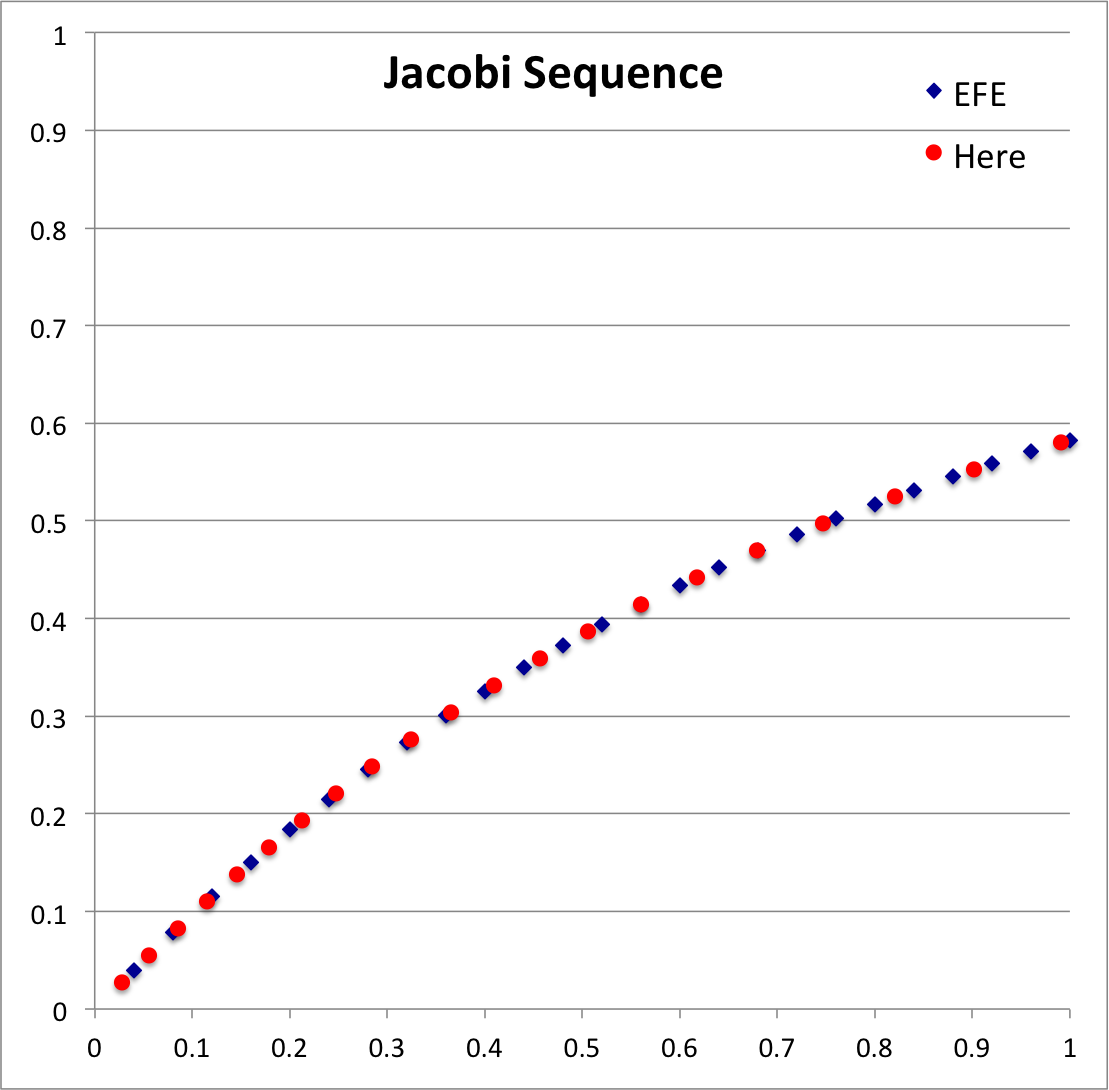
With regard to our Table 1 (immediately above): Given each pair of axis ratios, <math>~(\tfrac{b}{a},\tfrac{c}{a})</math> — copied from Table IV of EFE (see columns 1 and 2 of our Table 1) — and the corresponding coefficient values, <math>~A_1</math>, <math>~A_2</math>, and <math>~A_3</math>, as tabulated in Table 2 of our accompanying discussion, we calculated corresponding values of <math>~\Omega^2</math> (column 3) and total angular momentum (column 4) in the units used in EFE's Table IV, as well as (column 5) the total angular momentum in units used by Christodoulou, et al. (1995, ApJ, 446, 472) — see our related discussion of these physical quantities. We also have tabulated associated values of the function, <math>~f_J</math>, (column 6) and its first derivative, <math>~f_J^'</math>, (column 7) as defined immediately above. Notice that <math>~f_J</math> is very nearly zero in all cases, which indicates that each axis-ratio pair indeed identifies a configuration that lies along the Jacobi sequence.
|
Table 2: Jacobi Sequence |
|---|
b/a c/a 0.990699 0.580000 0.901558 0.552381 0.820783 0.524762 0.747135 0.497143 0.679613 0.469524 0.617393 0.441905 0.559798 0.414286 0.506257 0.386667 0.456291 0.359048 0.409492 0.331429 0.365507 0.303810 0.324034 0.276190 0.284807 0.248571 0.247591 0.220952 0.212179 0.193333 0.178382 0.165714 0.146026 0.138095 0.114948 0.110476 0.084989 0.082857 0.055982 0.055238 0.027738 0.027619 |
With regard to our Table 2 (immediately above): Here we specified twenty-one values of the axis ratio, <math>~\tfrac{c}{a}</math>, (column 2) and used our Newton-Raphson-based root finder to identify corresponding values of the companion axis ratio, <math>~\tfrac{b}{a}</math>, (column 1) that satisfies the governing relation, <math>~f_J = 0</math>.
Sequence Plots
| Jacobi Sequence: (blue) Points defined by data in Table IV of EFE, Chapter 6, §39 (p. 103); (red) points generated here from above-defined roots of the governing relation. |
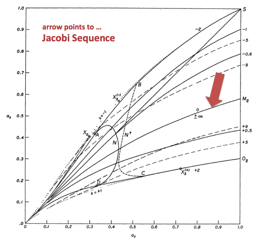
Figure 2 extracted† from p. 902 of S. Chandrasekhar (1965)
"The Equilibrium and the Stability of the Riemann Ellipsoids. I"
ApJ, vol. 142, pp. 890-921 © American Astronomical Society |
| †Original figure has been annotated (maroon-colored text and arrow added) for clarification. |
See Also

|
|---|
|
© 2014 - 2021 by Joel E. Tohline |

