Difference between revisions of "User:Tohline/Appendix/Ramblings/Azimuthal Distortions"
(→Empirical Construction of Eigenvector: Begin discussing empirical phase function) |
(Type in cautionary introductory paragraph) |
||
| (77 intermediate revisions by the same user not shown) | |||
| Line 2: | Line 2: | ||
<!-- __NOTOC__ will force TOC off --> | <!-- __NOTOC__ will force TOC off --> | ||
=Analyzing Azimuthal Distortions= | =Analyzing Azimuthal Distortions= | ||
<font color="red"><b>[Comment by J. E. Tohline on 24 May 2016]</b></font> This chapter contains a set of technical notes and accompanying discussion that I put together several months ago as I was trying to gain a foundational understanding of the results of a large study of instabilities in self-gravitating tori published by the Imamura & Hadley collaboration. I have come to appreciate that some of the logic and interpretation of published results that are presented, below, has serious flaws. Therefore, anyone reading this should be quite cautious in deciding what subsections provide useful insight. I have written a separate chapter titled, "[[User:Tohline/Apps/ImamuraHadleyCollaboration#Characteristics_of_Unstable_Eigenvectors_in_Self-Gravitating_Tori|Characteristics of Unstable Eigenvectors in Self-Gravitating Tori]]," that contains a much more trustworthy analysis of this very interesting problem. | |||
{{LSU_WorkInProgress}} | |||
{{LSU_HBook_header}} | {{LSU_HBook_header}} | ||
In what follows, we will draw heavily from | In what follows, we will draw heavily from three publications: (1) [http://adsabs.harvard.edu/abs/1990ApJ...361..394T J. E. Tohline & I. Hachisu (1990, ApJ, 361, 394-407)] — hereafter, TH90 — (2) [http://adsabs.harvard.edu/abs/1994ApJ...420..247W J. W. Woodward, J. E. Tohline, & I. Hachisu (1994, ApJ, 420, 247-267)] — hereafter, WTH94 — and (3) [http://adsabs.harvard.edu/abs/2011Ap%26SS.334....1H K. Hadley & J. N. Imamura (2011, ''Astrophysics and Space Science'', 334, 1)] — hereafter, HI11. | ||
==Adopted Notation== | ==Adopted Notation== | ||
Beginning with equation (2) of [http://adsabs.harvard.edu/abs/1990ApJ...361..394T | Beginning with equation (2) of [http://adsabs.harvard.edu/abs/1990ApJ...361..394T TH90] but ignoring variations in the vertical coordinate direction, the mass density is given by the expression, | ||
<div align="center"> | <div align="center"> | ||
<table border="0" cellpadding="5" align="center"> | <table border="0" cellpadding="5" align="center"> | ||
| Line 87: | Line 93: | ||
</div> | </div> | ||
Adopting [http://adsabs.harvard.edu/abs/1986PThPh..75. | Adopting [http://adsabs.harvard.edu/abs/1986PThPh..75..251K Kojima's (1986)] notation, that is, defining, | ||
<div align="center"> | <div align="center"> | ||
<table border="0" cellpadding="5" align="center"> | <table border="0" cellpadding="5" align="center"> | ||
| Line 157: | Line 163: | ||
whose relative amplitude — with a radial structure as specified inside the curly braces — is undergoing a uniform exponential growth but is otherwise unchanging. | whose relative amplitude — with a radial structure as specified inside the curly braces — is undergoing a uniform exponential growth but is otherwise unchanging. | ||
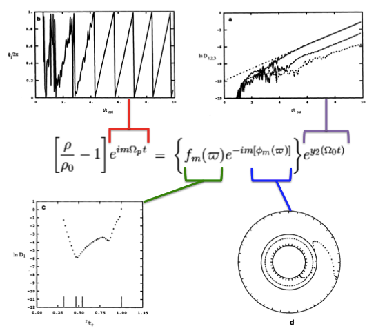
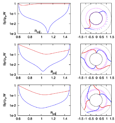
Drawing from figure 2 of [http://adsabs.harvard.edu/abs/ | Drawing from figure 2 of [http://adsabs.harvard.edu/abs/1994ApJ...420..247W WTH94], our Figure 1, immediately below, illustrates how the behavior of each factor in this expression can reveal itself during a numerical simulation that follows the time-evolutionary development of an unstable, nonaxisymmetric eigenmode. The initial model for this depicted evolution (model O3 from Table 1 of [http://adsabs.harvard.edu/abs/1994ApJ...420..247W WTH94]) is a zero-mass — that is, it is a [[User:Tohline/Apps/PapaloizouPringleTori#Massless_Polytropic_Tori|Papaloizou-Pringle like torus]] — with [[User:Tohline/SR#Barotropic_Structure|polytropic index]],<math>~n = 3</math>, and a rotation-law profile defined by [[User:Tohline/AxisymmetricConfigurations/SolutionStrategies#Simple_Rotation_Profile_and_Centrifugal_Potential|uniform specific angular momentum]]. | ||
* The top-left panel shows how, at any radial location, the phase angle, <math>~\phi_1/(2\pi)</math>, for the <math>~m=1</math> eigenmode, varies with time, <math>~t/t_\mathrm{rot}</math>, where, <math>~t_\mathrm{rot} \equiv 2\pi/\Omega_0</math> is the rotation period at the density maximum; | * The top-left panel shows how, at any radial location, the phase angle, <math>~\phi_1/(2\pi)</math>, for the <math>~m=1</math> eigenmode, varies with time, <math>~t/t_\mathrm{rot}</math>, where, <math>~t_\mathrm{rot} \equiv 2\pi/\Omega_0</math> is the rotation period at the density maximum; | ||
* Using a semi-log plot, the top-right panel shows the exponential growth of the amplitude of three separate modes: The dominant unstable mode, displaying the largest amplitude, is <math>~m = 1</math>. | * Using a semi-log plot, the top-right panel shows the exponential growth of the amplitude of three separate modes: The dominant unstable mode, displaying the largest amplitude, is <math>~m = 1</math>. | ||
* Using a semi-log plot (log amplitude versus fractional radius, <math>~\varpi/r_+</math>), the bottom-left panel displays the shape of the eigenfunction, <math>~f_1(\varpi)</math>, for the unstable, <math>~m=1</math> mode; | * Using a semi-log plot (log amplitude versus fractional radius, <math>~\varpi/r_+</math>), the bottom-left panel displays the shape of the eigenfunction, <math>~f_1(\varpi)</math>, for the unstable, <math>~m=1</math> mode; | ||
* The bottom-right panel displays the radial dependence of the equatorial-plane phase angle, <math>~\phi_1(\varpi)</math>, for the unstable, <math>~m=1</math> mode; this is what [http://adsabs.harvard.edu/abs/2011Ap%26SS.334....1H | * The bottom-right panel displays the radial dependence of the equatorial-plane phase angle, <math>~\phi_1(\varpi)</math>, for the unstable, <math>~m=1</math> mode; this is what [http://adsabs.harvard.edu/abs/2011Ap%26SS.334....1H HI11] refer to as the "constant phase locus." | ||
<div align="center"> | <div align="center" id="Figure1"> | ||
<table border="1" cellpadding="5" width="70%"> | <table border="1" cellpadding="5" width="70%"> | ||
<tr> | <tr> | ||
| Line 178: | Line 184: | ||
<tr> | <tr> | ||
<td align="center"> | <td align="center"> | ||
[[File:Diagram01.png| | [[File:Diagram01.png|550px|Rearranged Figure 2 from Woodward, Tohline, and Hachisu (1994)]] | ||
</td> | </td> | ||
</tr> | </tr> | ||
| Line 184: | Line 190: | ||
</table> | </table> | ||
</div> | </div> | ||
==Empirical Construction of Eigenvector== | ==Empirical Construction of Eigenvector== | ||
===Summary=== | |||
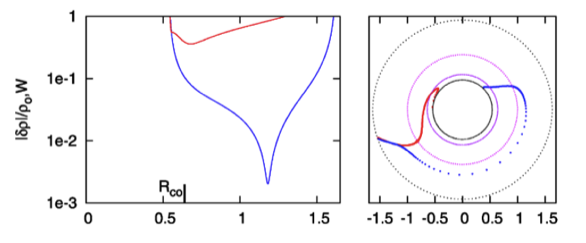
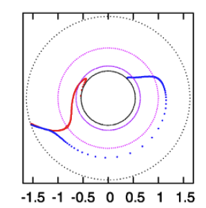
While studying the series of three papers that was published recently by the [[#See_Also|Imamura & Hadley collaboration]], I was particularly drawn to the pair of plots presented in Figure 6 — and, again, in the top portion of Figure 13 — of [http://adsabs.harvard.edu/abs/2011Ap%26SS.334....1H HI11]. This pair of plots has been reprinted here, without modification, as our Figure 2. As in the bottom two panels of our Figure 1, the curves delineated by the blue dots in this pair of [http://adsabs.harvard.edu/abs/2011Ap%26SS.334....1H HI11] plots display (on the left) the shape of the eigenfunction, <math>~f_1(\varpi)</math>, and (on the right) the "constant phase locus," <math>~\phi_1(\varpi)</math>, for an unstable, <math>~m=1</math> mode. In this case, the initial model for the depicted evolution is the equilibrium model from Table 2 of [http://adsabs.harvard.edu/abs/2011Ap%26SS.334....1H HI11] that has <math>~T/|W| = 0.253</math>; it is a fully self-gravitating torus with [[User:Tohline/SR#Barotropic_Structure|polytropic index]], <math>~n = 3/2</math>, and a rotation-law profile defined by a [[User:Tohline/AxisymmetricConfigurations/SolutionStrategies#Simple_Rotation_Profile_and_Centrifugal_Potential|"Keplerian" angular velocity profile]]. | |||
<div align="center"> | <div align="center"> | ||
<table border="1" cellpadding="3" align="center"> | <table border="1" cellpadding="3" align="center" width="60%"> | ||
<tr> | <tr> | ||
<td align="center"> | <td align="center"> | ||
| Line 198: | Line 204: | ||
</tr> | </tr> | ||
<tr><td align="center"> | <tr><td align="center"> | ||
Panel pair extracted<sup>†</sup> without modification from the top-most segment of Figure 13, p. 12 of [http://adsabs.harvard.edu/abs/2011Ap%26SS.334....1H K. Hadley & J. N. Imamura ( | Panel pair extracted<sup>†</sup> without modification from the top-most segment of Figure 13, p. 12 of [http://adsabs.harvard.edu/abs/2011Ap%26SS.334....1H K. Hadley & J. N. Imamura (2011)]<p></p> | ||
"''Nonaxisymmetric Instabilities of Self-Gravitating Disks. ''I'' Toroids''"<p></p> | "''Nonaxisymmetric Instabilities of Self-Gravitating Disks. ''I'' Toroids''"<p></p> | ||
''Astrophysics and Space Science'', 334, 1 - 26 © [http://www.springer.com/gp/about-springer/company-information/locations/springer-science-business-media-llc Springer Science+Business Media B.V.] | ''Astrophysics and Space Science'', 334, 1 - 26 © [http://www.springer.com/gp/about-springer/company-information/locations/springer-science-business-media-llc Springer Science+Business Media B.V.] | ||
</td></tr> | </td></tr> | ||
<tr><td align="center"> | <tr><td align="center"> | ||
[[File:ImamuraMontageTop.png|Comparison with Hadley & Imamura ( | [[File:ImamuraMontageTop.png|500px|Comparison with Hadley & Imamura (2011)]] | ||
</td></tr> | </td></tr> | ||
<tr><td align="left"><sup>†</sup>This pair of plots also appears, by itself, as Figure 6 on p. 12 of [http://adsabs.harvard.edu/abs/2011Ap%26SS.334....1H K. Hadley & J. N. Imamura ( | <tr><td align="left"><sup>†</sup>This pair of plots also appears, by itself, as Figure 6 on p. 12 of [http://adsabs.harvard.edu/abs/2011Ap%26SS.334....1H K. Hadley & J. N. Imamura (2011)].</td></tr> | ||
</table> | </table> | ||
</div> | </div> | ||
<div align="center" id="Figure3"> | |||
<table border="1" cellpadding="3" align="center" width="60%"> | |||
<tr> | |||
<td align="center"> | |||
<b><font size="+1">Figure 3:</font></b> | |||
Our Empirically Constructed Eigenvector | |||
</td> | |||
</tr> | |||
<tr><td align="center"> | |||
[[File:ImamuraMontage2Bottom.png|500px|Empirically Constructed Eigenfunction for Comparison with Imamura]] | |||
</td></tr> | |||
<tr><td align="left" colspan="2"> | |||
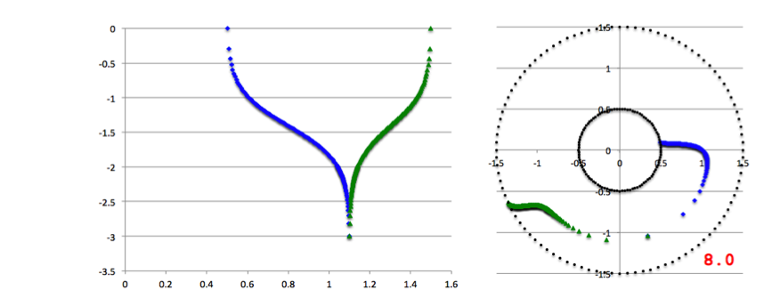
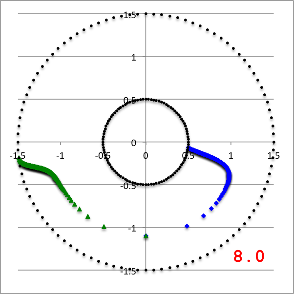
''Left panel'': A plot of our empirically constructed radial amplitude function, <math>~f_\ln(\varpi)</math>; the function has been normalized as explained in the boxed-in ''PRACTICAL IMPLEMENTATION'' remark, below. ''Right panel'': A plot of our empirically constructed phase function, <math>~\phi_1(\varpi)</math> with <math>~\aleph = 8.0</math>; after extraction from the animation sequence presented in Figure 4, here each point along this "constant phase locus" has been shifted by an additional phase of <math>~\pi/10</math> in order to better highlight its resemblance to the [http://adsabs.harvard.edu/abs/2011Ap%26SS.334....1H HI11] "constant phase locus" plot shown in the righthand panel of our Figure 2. In both panels, blue dots trace the function's behavior over the inner region of the torus <math>~(r_- < \varpi < r_\mathrm{mid})</math> and green dots trace the function's behavior over the outer region of the torus <math>~(r_\mathrm{mid} < \varpi < r_+)</math>. | |||
</td></tr> | |||
</table> | |||
</div> | |||
As is described in the subsections that follow, we have devised two related and relatively simple analytic expressions whose behaviors, as a function of <math>~\varpi</math>, qualitatively resemble the two blue, [http://adsabs.harvard.edu/abs/2011Ap%26SS.334....1H HI11] curves. Our two empirically constructed functions have been plotted in Figure 3, immediately below Figure 2, to aid visual comparison with the eigenfunctions that were generated by [http://adsabs.harvard.edu/abs/2011Ap%26SS.334....1H HI11] via a proper stability analysis. Next we describe the thought process that led to the construction of the amplitude and phase eigenfunctions presented in Figure 3. | |||
===Radial Eigenfunction=== | ===Radial Eigenfunction=== | ||
It occurred to me, first, that the blue curve displayed in the left-hand panel of [http://adsabs.harvard.edu/abs/2011Ap%26SS.334....1H | It occurred to me, first, that the blue curve displayed in the left-hand panel of [http://adsabs.harvard.edu/abs/2011Ap%26SS.334....1H HI11]'s figure 6 (our Figure 2) might be reasonably well approximated by piecing together a pair of arc-hyperbolic-tangent (ATANH) functions. In an effort to demonstrate this, I began by specifying a "midway" radial location, <math>~r_- < r_\mathrm{mid} < r_+ \, ,</math> at which the two ATANH functions meet and at which the density fluctuation is smallest. Then I defined a function of the form, | ||
<div align="center"> | <div align="center"> | ||
<table border="0" cellpadding="5" align="center"> | <table border="0" cellpadding="5" align="center"> | ||
| Line 217: | Line 244: | ||
<td align="center" bgcolor="blue"> </td> | <td align="center" bgcolor="blue"> </td> | ||
<td align="right"> | <td align="right"> | ||
<math>~ | <math>~f_\ln(\varpi)</math> | ||
</td> | </td> | ||
<td align="center"> | <td align="center"> | ||
| Line 236: | Line 263: | ||
<td align="center" bgcolor="green"> </td> | <td align="center" bgcolor="green"> </td> | ||
<td align="right"> | <td align="right"> | ||
<math>~ | <math>~f_\ln(\varpi)</math> | ||
</td> | </td> | ||
<td align="center"> | <td align="center"> | ||
| Line 254: | Line 281: | ||
</div> | </div> | ||
This empirically specified, two-piece <math>~ | This empirically specified, two-piece <math>~f_\ln(\varpi)</math> function has been plotted in the left-hand panel of Figure 3. (To facilitate quantitative comparison with Figure 2, the function has been normalized as explained in the boxed-in ''PRACTICAL IMPLEMENTATION'' remark that follows.) Blue dots trace the function's behavior over the lower radial-coordinate range while green dots trace its behavior over the upper radial-coordinate range. This plot of <math>~f_\ln(\varpi)</math> closely resembles the plot of the eigenfunction, <math>~\delta\rho/\rho (\varpi)</math> (see the left-hand panel of our Figure 2) that developed spontaneously via [http://adsabs.harvard.edu/abs/2011Ap%26SS.334....1H HI11]'s linear stability analysis. | ||
<div align="center"> | <div align="center"> | ||
<table border="1" cellpadding="3" align="center"> | <table border="1" cellpadding="3" align="center" width="50%"> | ||
<tr> | <tr><td align="left"> | ||
'''<font color="maroon">PRACTICAL IMPLEMENTATION:</FONT>''' At the two limits, <math>~\varpi = r_-</math> and <math>~\varpi = r_+</math>, the function, <math>~f_\ln(\varpi) \rightarrow +\infty</math>; while, at the limit, <math>~\varpi = r_\mathrm{mid}</math>, the function, <math>~f_\ln(\varpi) \rightarrow -\infty</math>. In practice, after dividing the relevant radial extent into 100 zones, we stay ''half of a radial zone'' away from these three limiting radial boundaries, so that the maximum and minimum values of <math>~f_\ln(\varpi)</math> are finite; specifically, in the example plotted here, we have set <math>~[f_\ln]_\mathrm{min} = -2.99448</math> and <math>~[f_\ln]_\mathrm{max} = 2.64665</math>. Then we strategically employ the finite values of the function at these near-boundary limits to rescale the function such that, in the plot shown here, it lies between -3 (minimum amplitude) and 0 (maximum amplitude). | |||
</ | |||
< | |||
[ | |||
</td></tr> | </td></tr> | ||
</table> | </table> | ||
| Line 272: | Line 293: | ||
<span id="SwitchToLog">Recognizing that the figure depicting</span> the [http://adsabs.harvard.edu/abs/2011Ap%26SS.334....1H HI11] eigenfunction is a semi-log plot, it seems clear that the relationship between our constructed function, <math>~f_\ln(\varpi)</math>, and the eigenfunction, <math>~f_1(\varpi)</math>, is, | |||
<div align="center"> | <div align="center"> | ||
<math>~f_1(\varpi) = e^{f_\ln(\varpi)} \, .</math> | |||
</div> | </div> | ||
Now, in general, the following mathematical relation holds: | |||
Now, the following | |||
<div align="center"> | <div align="center"> | ||
<table border="0" cellpadding="5" align="center"> | <table border="0" cellpadding="5" align="center"> | ||
| Line 294: | Line 309: | ||
</td> | </td> | ||
<td align="left"> | <td align="left"> | ||
<math>~ | <math>~\ln\biggl( \frac{1+x}{1-x} \biggr)^{1/2} </math> | ||
</td> | </td> | ||
<td align="center"> | <td align="center"> | ||
| Line 365: | Line 380: | ||
</table> | </table> | ||
</div> | </div> | ||
Therefore we can write, | <span id="SquareRoot">Therefore we can write,</span> | ||
<div align="center"> | <div align="center"> | ||
<table border="0" cellpadding="5" align="center"> | <table border="0" cellpadding="5" align="center"> | ||
| Line 372: | Line 387: | ||
<td align="center" bgcolor="blue"> </td> | <td align="center" bgcolor="blue"> </td> | ||
<td align="right"> | <td align="right"> | ||
<math>~ | <math>~f_1(\varpi) = e^{f_\ln(\varpi)}</math> | ||
</td> | </td> | ||
<td align="center"> | <td align="center"> | ||
| Line 378: | Line 393: | ||
</td> | </td> | ||
<td align="left"> | <td align="left"> | ||
<math>~ | <math>~\biggl( \frac{r_\mathrm{mid} - \varpi}{\varpi - r_-} \biggr)^{1/2} | ||
</math> | </math> | ||
</td> | </td> | ||
| Line 385: | Line 400: | ||
</td> | </td> | ||
<td align="left"> | <td align="left"> | ||
<math>r_- < \varpi < r_\mathrm{mid} \, | <math>r_- < \varpi < r_\mathrm{mid} \, .</math> | ||
</td> | </td> | ||
</tr> | </tr> | ||
</table> | </table> | ||
</div> | </div> | ||
Similarly, we find that, over the upper radial-coordinate range, | |||
<div align="center"> | <div align="center"> | ||
<table border="0" cellpadding="5" align="center"> | <table border="0" cellpadding="5" align="center"> | ||
| Line 397: | Line 412: | ||
<td align="center" bgcolor="green"> </td> | <td align="center" bgcolor="green"> </td> | ||
<td align="right"> | <td align="right"> | ||
<math>~ | <math>~f_1(\varpi) = e^{f_\ln(\varpi)}</math> | ||
</td> | </td> | ||
<td align="center"> | <td align="center"> | ||
| Line 403: | Line 418: | ||
</td> | </td> | ||
<td align="left"> | <td align="left"> | ||
<math>~ | <math>~\biggl( \frac{r_\mathrm{mid} - \varpi}{\varpi - r_+} \biggr)^{1/2} | ||
</math> | </math> | ||
</td> | </td> | ||
| Line 416: | Line 431: | ||
</div> | </div> | ||
===Constant Phase Loci=== | |||
Now let's work on the phase function, <math>~\phi_1(\varpi)</math>. The phase function displayed in the right-hand panel of our Figure 2 — that is, the phase function that developed spontaneously from the linear stability analysis performed by [http://adsabs.harvard.edu/abs/2011Ap%26SS.334....1H HI11] — appears to be fairly constant (''i.e.,'' the phase is independent of radius) in the innermost region of the torus and, then again, fairly constant in the outermost region of the torus with a smooth but fairly rapid phase shift of approximately <math>~\pi</math> radians between the two extremes. This is the behavior exhibited by an arctangent (ATAN) function. With this in mind, we have defined a new function, <math>~D(\varpi)</math>, ''in terms of'' our empirically derived radial eigenfunction, <math>~f_\ln(\varpi)</math>, as follows: | |||
Now let's work on the phase function, <math>~\phi_1(\varpi)</math>. The phase function displayed in the right-hand panel of our Figure 2 — that is, the phase function that developed spontaneously from [http://adsabs.harvard.edu/abs/2011Ap%26SS.334....1H | |||
<div align="center"> | <div align="center"> | ||
| Line 431: | Line 446: | ||
</td> | </td> | ||
<td align="left"> | <td align="left"> | ||
<math>~\frac{ | <math>~\frac{f_\ln(\varpi) - [f_\ln]_\mathrm{min}}{[f_\ln]_\mathrm{max} - [f_\ln]_\mathrm{min}} \, .</math> | ||
</td> | </td> | ||
</tr> | </tr> | ||
| Line 437: | Line 452: | ||
</div> | </div> | ||
It has the following behavior: | |||
* At the inner edge of the torus <math>~(r_-)</math>, where <math>~f_\ln(\varpi) = [f_\ln]_\mathrm{max}</math>, <math>~D(\varpi) = 1</math>; | |||
* At <math>~r_\mathrm{mid}</math>, where <math>~f_\ln(\varpi) = [f_\ln]_\mathrm{min}</math>, <math>~D(\varpi) = 0</math>; | |||
* At the outer edge of the torus <math>~(r_+)</math>, where again <math>~f_\ln(\varpi) = [f_\ln]_\mathrm{max}</math>, <math>~D(\varpi) = 1</math>. | |||
This function can therefore satisfactorily serve as an argument of the ATAN function, swinging the phase by <math>~\pi/2</math> over the inner (blue) region of the torus, then swinging the phase by an additional <math>~\pi/2</math> over the outer (green) region of the torus. If we furthermore multiply the function by a variable coefficient — call it, <math>~\aleph</math> — before feeding it to the ATAN function, we can adjust the thickness of the radial domain over which the total phase transition occurs. What appears to work well is the following: | |||
<div align="center"> | |||
<table border="0" cellpadding="5" align="center"> | |||
<tr> | |||
<td align="center" bgcolor="blue"> </td> | |||
<td align="right"> | |||
<math>~\phi_1(\varpi) + \frac{\pi}{2} </math> | |||
</td> | |||
<td align="center"> | |||
<math>~=</math> | |||
</td> | |||
<td align="left"> | |||
<math>~+~\tan^{-1}[\aleph \cdot D(\varpi)]</math> | |||
</td> | |||
<td align="center"> | |||
for | |||
</td> | |||
<td align="left"> | |||
<math>r_- < \varpi < r_\mathrm{mid} \, ;</math> | |||
</td> | |||
</tr> | |||
</table> | |||
</div> | |||
and | |||
<div align="center"> | |||
<table border="0" cellpadding="5" align="center"> | |||
<tr> | |||
<td align="center" bgcolor="green"> </td> | |||
<td align="right"> | |||
<math>~\phi_1(\varpi) + \frac{\pi}{2} </math> | |||
</td> | |||
<td align="center"> | |||
<math>~=</math> | |||
</td> | |||
<td align="left"> | |||
<math>~-~\tan^{-1}[\aleph \cdot D(\varpi)] </math> | |||
</td> | |||
<td align="center"> | |||
for | |||
</td> | |||
<td align="left"> | |||
<math>r_\mathrm{mid} < \varpi < r_+ \, .</math> | |||
</td> | |||
</tr> | |||
</table> | |||
</div> | |||
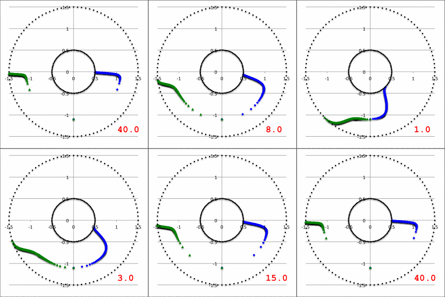
In the lefthand panel of Figure 4, the "constant phase loci" defined by this empirically constructed phase function have been mapped onto a polar-coordinate grid for ten different values of the leading coefficient in the range, <math>~1.0 \le \aleph \le 40.0</math>, as recorded in the bottom-right corner of the plot. The constant phase locus created by setting <math>~\aleph = 8.0</math> has been singled out and displayed in the middle panel of Figure 4, because it closely resembles the "constant phase locus" published by HI11a (reprinted here as the righthand panel of Figure 4 to facilitate comparison). | |||
<table border="1" cellpadding="8" align="center"> | |||
<tr><th align="center" colspan="3"><font size="+1">Figure 4</font></th></tr> | |||
<tr> | |||
<td align="center" colspan="2">Constant Phase Loci Generated by Our Empirically Constructed Phase Function, <math>~\phi_1(\varpi)</math></td> | |||
<td align="center" rowspan="2">[http://adsabs.harvard.edu/abs/2011Ap%26SS.334....1H HI11]'s Published Constant Phase Loci</td> | |||
</tr> | |||
<tr><td align="center">Ten Values of <math>~\aleph</math></td><td align="center">For <math>~\aleph = 8</math></td></tr> | |||
<tr> | |||
<td align="center"> | |||
[[File:ImamuraPhaseMovie.gif|230px|Movie Showing Empirically Constructed Phase]] | |||
</td> | |||
<td align="center"> | |||
[[File:a05.png|230px|Best Match]] | |||
</td> | |||
<td align="center"> | |||
[[File:ImamuraOriginalPhase.png|250px|HI11a constant phase loci]] | |||
</td> | |||
</tr> | |||
</table> | |||
<!-- | |||
Then we set, | Then we set, | ||
<div align="center"> | <div align="center"> | ||
<table border="0" cellpadding="5" align="center"> | <table border="0" cellpadding="5" align="center"> | ||
| Line 450: | Line 543: | ||
</td> | </td> | ||
<td align="left"> | <td align="left"> | ||
<math>~\biggl\{\tan^{-1}[ | <math>~\biggl\{\tan^{-1}[\aleph \cdot D(\varpi)] - \frac{\pi}{2} \biggr\} + \frac{\pi}{10} \, .</math> | ||
</td> | </td> | ||
</tr> | </tr> | ||
| Line 456: | Line 549: | ||
</div> | </div> | ||
Now | Now — as stated earlier in the [[#Figure3|caption to Figure 3]] — for the specific case being graphically illustrated here, <math>~[f_\ln]_\mathrm{min} = -2.99448</math> and <math>~[f_\ln]_\mathrm{max} = 2.64665</math>. Hence, | ||
<div align="center"> | <div align="center"> | ||
| Line 469: | Line 562: | ||
</td> | </td> | ||
<td align="left"> | <td align="left"> | ||
<math>~\tan^{-1}\biggl | <math>~\tan^{-1}\biggl\{8\cdot \biggl[ | ||
\frac{f_\ln(\varpi) - [f_\ln]_\mathrm{min}}{[f_\ln]_\mathrm{max} - [f_\ln]_\mathrm{min}} | |||
\biggr]\biggr\} | |||
</math> | </math> | ||
</td> | </td> | ||
| Line 489: | Line 584: | ||
</div> | </div> | ||
where, <math>~a = 1.41816</math> and <math>~b = 4.24664</math>. | where, <math>~a = 1.41816</math> and <math>~b = 4.24664</math>. | ||
--> | |||
==Discussion== | |||
===Simpler Connection Between Radial and Phase Eigenfunctions=== | |||
When it is used as an argument of ATAN, the function, <math>~D(\varpi)</math>, [[#Constant_Phase_Loci|as defined above]] smoothly steers <math>~\phi_1</math> through a phase shift of approximately <math>~\pi</math> radians principally because the function itself smoothly varies between <math>~+1</math> and <math>~0</math> (then back again). Let's play with some simpler expressions for this governing function that also vary smoothly between these limits. | |||
Define, | |||
<div align="center"> | |||
<table border="0" cellpadding="5" align="center"> | |||
<tr> | |||
<td align="right"> | |||
<math>~\Delta_\mathrm{inner}</math> | |||
</td> | |||
<td align="center"> | |||
<math>~\equiv</math> | |||
</td> | |||
<td align="left"> | |||
<math>~\biggl( \frac{\varpi - r_-}{r_\mathrm{mid}-r_-} \biggr)</math> | |||
</td> | |||
<td align="center"> | |||
has range of | |||
</td> | |||
<td align="left"> | |||
<math>~+0 ~~\rightarrow ~~ +1 \, ;</math> | |||
</td> | |||
</tr> | |||
<tr> | |||
<td align="right"> | |||
<math>~\Delta_\mathrm{outer}</math> | |||
</td> | |||
<td align="center"> | |||
<math>~\equiv</math> | |||
</td> | |||
<td align="left"> | |||
<math>~\biggl( \frac{\varpi - r_+}{r_\mathrm{mid}-r_+} \biggr)</math> | |||
</td> | |||
<td align="center"> | |||
has range of | |||
</td> | |||
<td align="left"> | |||
<math>~+1 ~~\rightarrow ~~ +0 \, .</math> | |||
</td> | |||
</tr> | |||
</table> | |||
</div> | |||
The argument of ATANH, [[#Radial_Eigenfunction|as presented above]], was obtained from this relatively simple expression via the shift, | |||
<div align="center"> | |||
<table border="0" cellpadding="5" align="center"> | |||
<tr> | |||
<td align="right"> | |||
<math>~1-2\Delta_\mathrm{inner}</math> | |||
</td> | |||
<td align="center"> | |||
<math>~\equiv</math> | |||
</td> | |||
<td align="left"> | |||
<math>~\biggl( \frac{\varpi - r_-}{r_\mathrm{mid}-r_-} \biggr)</math> | |||
</td> | |||
<td align="center"> | |||
has range of | |||
</td> | |||
<td align="left"> | |||
<math>~+1 ~~\rightarrow ~~ -1 \, ;</math> | |||
</td> | |||
</tr> | |||
<tr> | |||
<td align="right"> | |||
<math>~1-2\Delta_\mathrm{outer}</math> | |||
</td> | |||
<td align="center"> | |||
<math>~\equiv</math> | |||
</td> | |||
<td align="left"> | |||
<math>~\biggl( \frac{\varpi - r_+}{r_\mathrm{mid}-r_+} \biggr)</math> | |||
</td> | |||
<td align="center"> | |||
has range of | |||
</td> | |||
<td align="left"> | |||
<math>~-1 ~~\rightarrow ~~ +1 \, .</math> | |||
</td> | |||
</tr> | |||
</table> | |||
</div> | |||
For the argument of <math>~D(\varpi)</math> function, we could therefore use, | |||
<div align="center"> | |||
<table border="0" cellpadding="5" align="center"> | |||
<tr> | |||
<td align="right"> | |||
<math>~1-\Delta_\mathrm{inner}</math> | |||
</td> | |||
<td align="center"> | |||
<math>~\equiv</math> | |||
</td> | |||
<td align="left"> | |||
<math>~\biggl( \frac{\varpi - r_-}{r_\mathrm{mid}-r_-} \biggr)</math> | |||
</td> | |||
<td align="center"> | |||
has range of | |||
</td> | |||
<td align="left"> | |||
<math>~+1 ~~\rightarrow ~~ 0 \, ;</math> | |||
</td> | |||
</tr> | |||
<tr> | |||
<td align="right"> | |||
<math>~1-\Delta_\mathrm{outer}</math> | |||
</td> | |||
<td align="center"> | |||
<math>~\equiv</math> | |||
</td> | |||
<td align="left"> | |||
<math>~\biggl( \frac{\varpi - r_+}{r_\mathrm{mid}-r_+} \biggr)</math> | |||
</td> | |||
<td align="center"> | |||
has range of | |||
</td> | |||
<td align="left"> | |||
<math>~0 ~~\rightarrow ~~ +1 \, .</math> | |||
</td> | |||
</tr> | |||
</table> | |||
</div> | |||
===Playing with the Radial Eigenfunction=== | |||
Up to this point, we've only considered radial eigenfunctions composed of two components (a "blue" inner component and a "green" outer component) that do not overlap. Here we'll allow the two components to overlap by assigning different values of <math>~r_\mathrm{mid}</math> to the two separate components — more specifically, we'll allow <math>~r_\mathrm{mid}|_\mathrm{green} \le r_\mathrm{mid}|_\mathrm{blue}</math> — then add the two functions over the region of overlap. Let's consider components of the following form: | |||
<div align="center"> | |||
<table border="0" cellpadding="5" align="center"> | |||
<tr> | |||
<td align="center" bgcolor="blue"> </td> | |||
<td align="right"> | |||
<math>~f_\mathrm{blue}(\varpi) </math> | |||
</td> | |||
<td align="center"> | |||
<math>~=</math> | |||
</td> | |||
<td align="left"> | |||
<math>~\biggl( \frac{r_\mathrm{blue} - \varpi}{\varpi - r_-} \biggr)^{p} | |||
</math> | |||
</td> | |||
<td align="center"> | |||
for | |||
</td> | |||
<td align="left"> | |||
<math>r_- < \varpi < r_\mathrm{blue} \, ,</math> | |||
</td> | |||
</tr> | |||
</table> | |||
</div> | |||
and, | |||
<div align="center"> | |||
<table border="0" cellpadding="5" align="center"> | |||
<tr> | |||
<td align="center" bgcolor="green"> </td> | |||
<td align="right"> | |||
<math>~f_\mathrm{green}(\varpi) </math> | |||
</td> | |||
<td align="center"> | |||
<math>~=</math> | |||
</td> | |||
<td align="left"> | |||
<math>~\biggl( \frac{r_\mathrm{green} - \varpi}{\varpi - r_+} \biggr)^{p} | |||
</math> | |||
</td> | |||
<td align="center"> | |||
for | |||
</td> | |||
<td align="left"> | |||
<math>r_\mathrm{green} < \varpi < r_+ \, ,</math> | |||
</td> | |||
</tr> | |||
</table> | |||
</div> | |||
where, <math>~p</math> is a exponent yet to be specified. So, for fixed values of the inner and outer radii of the torus, <math>~r_-</math> and <math>~r_+</math>, this two-component function has three adjustable variables. They are, <math>~r_\mathrm{blue}</math>, <math>~r_\mathrm{green}</math>, and <math>~p</math>. | |||
====Experimenting==== | |||
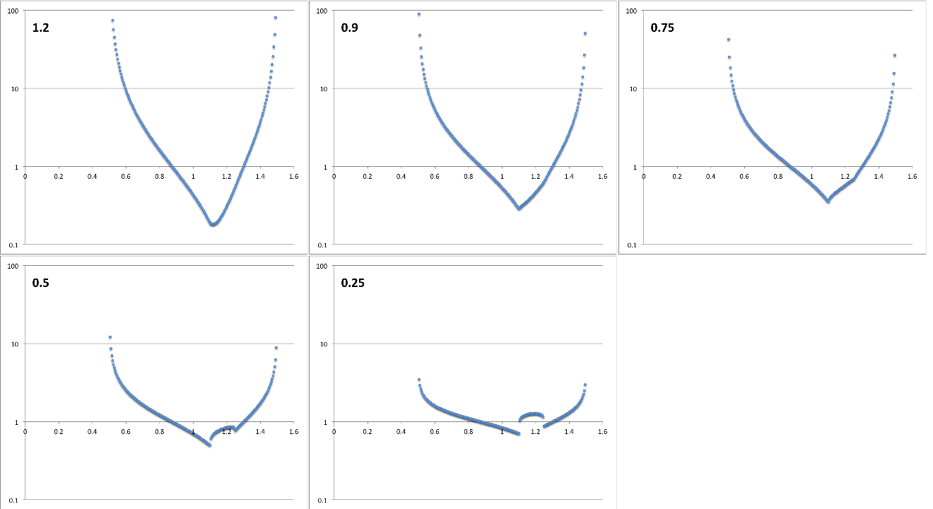
In Figure 5, <math>~r_\mathrm{blue}</math> and <math>~r_\mathrm{green}</math> are fixed, and <math>~p</math> is varied. | |||
<div align="center"> | |||
<table border="1" align="center" cellpadding="5" width="80%"> | |||
<tr> | |||
<th align="center"><font size="+1">Figure 5:</font> Variable exponent, <math>~p</math></th> | |||
</tr> | |||
<tr><td align="center"> | |||
<math>~r_- = 0.5</math>, <math>~r_+ = 1.5</math> | |||
… | |||
<math>~r_\mathrm{blue} = 1.25</math>, <math>~r_\mathrm{green}= 1.1</math> | |||
</td></tr> | |||
<tr><td align="center"> | |||
[[File:MontageAbrief.png|500px|Playing with radial eigenfunction]] | |||
</td></tr> | |||
<tr><td align="left"> | |||
In this example, the exponent, <math>~p</math>, is varied over the range, <math>~0.25 \le p \le 1.2</math>, as indicated by the numerical values shown in the upper-lefthand corner of each panel. | |||
</td></tr> | |||
</table> | |||
</div> | |||
Based on the [[#SquareRoot|above discussion]], I expected that the best match to the eigenfunctions found in [http://adsabs.harvard.edu/abs/2011Ap%26SS.334....1H HI11] would be <math>~p=0.5</math>, that is, a square-root. However, as illustrated in Figure 5, this and other fractional exponents less than unity generate noncontinuous derivatives at the overlapping edges of our two-piece function. Instead, a value of <math>~p = 1.2</math> seems to exhibit a more desired, smooth behavior. | |||
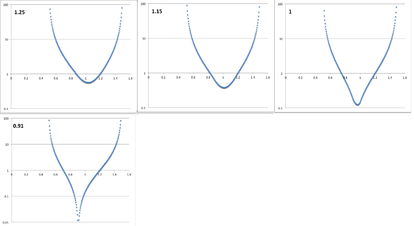
In Figure 6, <math>~r_\mathrm{green}</math> and <math>~p</math> are fixed, and <math>~r_\mathrm{blue}</math> is varied. | |||
<div align="center"> | |||
<table border="1" align="center" cellpadding="5" width="80%"> | |||
<tr> | |||
<th align="center"><font size="+1">Figure 6:</font> Variable <math>~r_\mathrm{blue}</math></th> | |||
</tr> | |||
<tr><td align="center"> | |||
<math>~r_- = 0.5</math>, <math>~r_+ = 1.5</math> | |||
… | |||
<math>~p = 1.2</math>, <math>~r_\mathrm{green}= 0.9</math> | |||
</td></tr> | |||
<tr><td align="center"> | |||
[[File:MontageBbrief.png|500px|Playing with radial eigenfunction]] | |||
</td></tr> | |||
<tr><td align="left"> | |||
In this example, the "blue" edge is varied over the range, <math>~0.91 \le r_\mathrm{blue} \le 1.25</math>, as indicated by the numerical values shown in the upper-lefthand corner of each panel. | |||
</td></tr> | |||
</table> | |||
</div> | |||
The frames of Figure 6 illustrate the qualitative behavior we have been seeking. Setting the exponent, <math>~p</math>, to a value greater than unity then varying one of the edges of the two-part eigenfunction provides a natural variation from "pointed" curves that look like adjoined arc-hyperbolic tangents to others that look more like a parabola. | |||
====Trial Comparison with HI11==== | |||
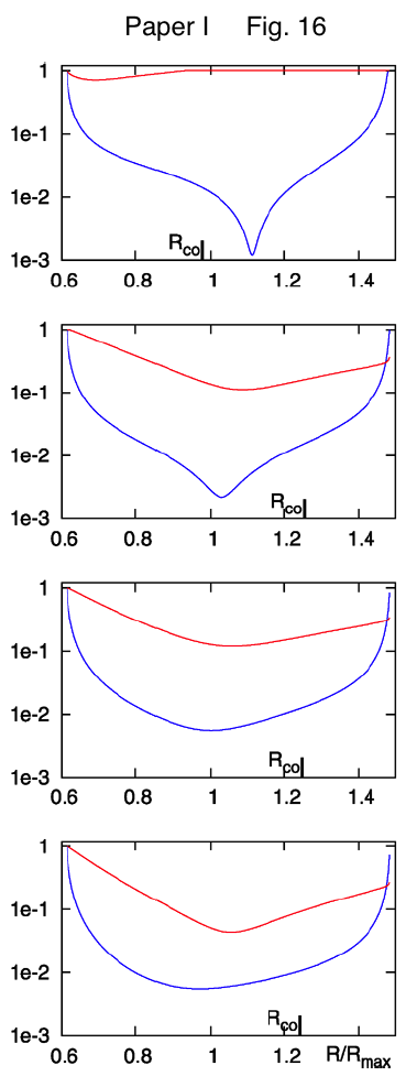
In Figure 7, we show how a straightforward, smooth adjustment of one parameter — namely, <math>~r_\mathrm{blue}</math> — generates a series of eigenfunctions that nicely match the set of radial eigenfunctions that are displayed in Figure 16 of [http://adsabs.harvard.edu/abs/2011Ap%26SS.334....1H HI11]. | |||
<div align="center" id="Figure7"> | |||
<table border="1" cellpadding="3" align="center" width="60%"> | |||
<tr> | |||
<td align="center" colspan="2"> | |||
<b><font size="+1">Figure 7:</font></b> | |||
Radial Eigenfunction Comparison | |||
</td> | |||
</tr> | |||
<tr> | |||
<td align="center">'''(a)''' Extracted from Figure 16 of [http://adsabs.harvard.edu/abs/2011Ap%26SS.334....1H HI11]</td> | |||
<td align="center">'''(b)''' Our Empirically Constructed Function</td> | |||
</tr> | |||
<tr><td align="center" rowspan="4"> | |||
[[File:PaperI_Fig16.png|300px|Figure 16 from HI11]] | |||
</td><td align="center">[[File:PhaseMovieFrameFirst.png|250px|Figure 16 from HI11]] | |||
</td></tr> | |||
<tr><td align="center">[[File:EigenfunctionMovie01.gif|250px|Figure 16 from HI11]]</td></tr> | |||
<tr><td align="center">[[File:PhaseMovieFrameLast.png|250px|Figure 16 from HI11]]</td></tr> | |||
<tr> | |||
<td align="left" colspan="1"> | |||
Here we set <math>~r_- = 0.6</math>, <math>~r_+ = 1.5</math>, <math>~r_\mathrm{blue}= 1.15</math>, and | |||
<math>~p = 1.2</math>, then let the "green" edge vary over the range, <math>~0.605 \le r_\mathrm{green} \le 1.144</math>. Via an animation, the middle panel illustrates the behavior of our empirically constructed eigenfunction over this entire range of values as indicated by the numerical value shown in the bottom-righthand corner of the panel; the top and bottom panels display the shape of our eigenfunction at the two extreme values of <math>~r_\mathrm{green}</math>. | |||
</td> | |||
</tr> | |||
</table> | |||
</div> | |||
===Relationship to Fourier Series Amplitude and Phase=== | |||
Recalling that, | |||
<div align="center"> | |||
<table border="0" cellpadding="5" align="center"> | |||
<tr> | |||
<td align="right"> | |||
<math>~e^{i\alpha}</math> | |||
</td> | |||
<td align="center"> | |||
<math>~=</math> | |||
</td> | |||
<td align="left"> | |||
<math>~\cos\alpha + i\sin\alpha \, ,</math> | |||
</td> | |||
</tr> | |||
</table> | |||
</div> | |||
we appreciate that the real part of the amplitude term — the term inside the curly braces of the expression found in [[#Figure1|Figure 1, above]] — can be written as, | |||
<div align="center"> | |||
<table border="0" cellpadding="5" align="center"> | |||
<tr> | |||
<td align="right"> | |||
<math>~\mathcal{A}_m \equiv \Re\{f_m e^{im\phi}\}</math> | |||
</td> | |||
<td align="center"> | |||
<math>~=</math> | |||
</td> | |||
<td align="left"> | |||
<math>~f_m \cos(m\phi_m) \, .</math> | |||
</td> | |||
</tr> | |||
</table> | |||
</div> | |||
When viewed in the context of a discrete Fourier series, we also recognize that the two functions, <math>~f_m</math> and <math>~\phi_m</math>, can be transformed into the pair of amplitude functions, | |||
<div align="center"> | |||
<table border="0" cellpadding="5" align="center"> | |||
<tr> | |||
<td align="right"> | |||
<math>~f_m ~~~\rightarrow ~~~ (a_m^2 + b_m^2)^{1/2}</math> | |||
</td> | |||
<td align="center"> | |||
| |||
and | |||
| |||
</td> | |||
<td align="left"> | |||
<math>~m\phi_m ~~~\rightarrow ~~~ \tan^{-1}\biggl(-\frac{b_m}{a_m}\biggr) \, ;</math> | |||
</td> | |||
</tr> | |||
</table> | |||
</div> | |||
that is, | |||
<div align="center"> | |||
<table border="0" cellpadding="5" align="center"> | |||
<tr> | |||
<td align="right"> | |||
<math>~a_m ~=~ f_m\cos(m\phi_m)</math> | |||
</td> | |||
<td align="center"> | |||
| |||
and | |||
| |||
</td> | |||
<td align="left"> | |||
<math>~b_m ~=~ -f_m\sin(m\phi_m) \, .</math> | |||
</td> | |||
</tr> | |||
</table> | |||
</div> | |||
Let's see where these expression lead us, given our above-adopted expressions for <math>~f_m</math> and <math>~\phi_m</math>. Given, | |||
<div align="center"> | |||
<table border="0" cellpadding="5" align="center"> | |||
<tr> | |||
<td align="right"> | |||
<math>~f = e^{f_\ln}</math> | |||
</td> | |||
<td align="center"> | |||
<math>~=</math> | |||
</td> | |||
<td align="left"> | |||
<math>~\biggl( \frac{r_\mathrm{blue} - \varpi}{\varpi - r_-} \biggr)^{p} \, ,</math> | |||
</td> | |||
</tr> | |||
</table> | |||
</div> | |||
and, | |||
<div align="center"> | |||
<table border="0" cellpadding="5" align="center"> | |||
<tr> | |||
<td align="right"> | |||
<math>~m\phi_m</math> | |||
</td> | |||
<td align="center"> | |||
<math>~=</math> | |||
</td> | |||
<td align="left"> | |||
<math>~\tan^{-1}[\aleph \cdot D(\varpi)] \, </math> | |||
</td> | |||
</tr> | |||
</table> | |||
</div> | |||
where, | |||
<div align="center"> | |||
<table border="0" cellpadding="5" align="center"> | |||
<tr> | |||
<td align="right"> | |||
<math>~D(\varpi)</math> | |||
</td> | |||
<td align="center"> | |||
<math>~=</math> | |||
</td> | |||
<td align="left"> | |||
<math>~\frac{f_\ln(\varpi) - [f_\ln]_\mathrm{min}}{[f_\ln]_\mathrm{max} - [f_\ln]_\mathrm{min}} \, ,</math> | |||
</td> | |||
</tr> | |||
</table> | |||
</div> | |||
we have, | |||
<div align="center"> | |||
<table border="0" cellpadding="5" align="center"> | |||
<tr> | |||
<td align="right"> | |||
<math>~a_m</math> | |||
</td> | |||
<td align="center"> | |||
<math>~=</math> | |||
</td> | |||
<td align="left"> | |||
<math>~ | |||
\biggl( \frac{r_\mathrm{blue} - \varpi}{\varpi - r_-} \biggr)^{p} | |||
\cos\biggl[ \tan^{-1}\biggl( \aleph \cdot D \biggr) \biggr] | |||
</math> | |||
</td> | |||
</tr> | |||
<tr> | |||
<td align="right"> | |||
| |||
</td> | |||
<td align="center"> | |||
<math>~=</math> | |||
</td> | |||
<td align="left"> | |||
<math>~ | |||
e^{f_\ln} \biggl[ 1+(\aleph \cdot D )^2 \biggr]^{-1/2} | |||
</math> | |||
</td> | |||
</tr> | |||
<tr> | |||
<td align="right"> | |||
| |||
</td> | |||
<td align="center"> | |||
<math>~=</math> | |||
</td> | |||
<td align="left"> | |||
<math>~ | |||
e^{f_\ln} \bigg\{ 1+\aleph^2_\mathrm{norm} \biggl( f_\ln(\varpi) - [f_\ln]_\mathrm{min} \biggr)^2 \biggr\}^{-1/2} \, , | |||
</math> | |||
</td> | |||
</tr> | |||
</table> | |||
</div> | |||
where, | |||
<div align="center"> | |||
<math>~\aleph_\mathrm{norm} \equiv \frac{\aleph}{[f_\ln]_\mathrm{max} - [f_\ln]_\mathrm{min}} \, .</math> | |||
</div> | |||
===Another Improvement=== | |||
I've realized that the phase plot is much smoother — in particular, the derivatives of both segments appear to match at their point of intersection — if we use <math>~D^{1/2}</math>, instead of simply <math>~D</math>, as the argument of the arctangent function. So, we define, | |||
<div align="center"> | |||
<table border="0" cellpadding="5" align="center"> | |||
<tr> | |||
<td align="right"> | |||
<math>~D_{1/2}(\varpi)</math> | |||
</td> | |||
<td align="center"> | |||
<math>~\equiv</math> | |||
</td> | |||
<td align="left"> | |||
<math>~\sqrt{D(\varpi)} = \biggl[ \frac{f_\ln(\varpi) - [f_\ln]_\mathrm{min}}{[f_\ln]_\mathrm{max} - [f_\ln]_\mathrm{min}} \biggr]^{1/2} \, ,</math> | |||
</td> | |||
</tr> | |||
</table> | |||
</div> | |||
and henceforth will set, | |||
<div align="center"> | |||
<table border="1" cellpadding="8" align="center"> | |||
<tr><td align="center"> | |||
<table border="0" cellpadding="5" align="center"> | |||
<tr> | |||
<td align="right"> | |||
<math>~m\phi_m</math> | |||
</td> | |||
<td align="center"> | |||
<math>~=</math> | |||
</td> | |||
<td align="left"> | |||
<math>~\pm \tan^{-1}[\aleph \cdot D_{1/2}(\varpi)] \, .</math> | |||
</td> | |||
</tr> | |||
</table> | |||
</td></tr> | |||
</table> | |||
</div> | |||
With this new argument for the arctangent function, we have, | |||
<div align="center"> | |||
<table border="0" cellpadding="5" align="center"> | |||
<tr> | |||
<td align="right"> | |||
<math>~a_m</math> | |||
</td> | |||
<td align="center"> | |||
<math>~=</math> | |||
</td> | |||
<td align="left"> | |||
<math>~ | |||
\biggl( \frac{r_\mathrm{blue} - \varpi}{\varpi - r_-} \biggr)^{p} | |||
\cos\biggl[ \tan^{-1}\biggl( \aleph \cdot D_{1/2} \biggr) \biggr] | |||
</math> | |||
</td> | |||
</tr> | |||
<tr> | |||
<td align="right"> | |||
| |||
</td> | |||
<td align="center"> | |||
<math>~=</math> | |||
</td> | |||
<td align="left"> | |||
<math>~ | |||
e^{f_\ln} \biggl[ 1+(\aleph \cdot D_{1/2} )^2 \biggr]^{-1/2} | |||
</math> | |||
</td> | |||
</tr> | |||
<tr> | |||
<td align="right"> | |||
| |||
</td> | |||
<td align="center"> | |||
<math>~=</math> | |||
</td> | |||
<td align="left"> | |||
<math>~ | |||
e^{f_\ln} \bigg\{ 1+\aleph^2_\mathrm{norm} \biggl( f_\ln(\varpi) - [f_\ln]_\mathrm{min} \biggr) \biggr\}^{-1/2} | |||
</math> | |||
</td> | |||
</tr> | |||
<tr> | |||
<td align="right"> | |||
| |||
</td> | |||
<td align="center"> | |||
<math>~=</math> | |||
</td> | |||
<td align="left"> | |||
<math>~ | |||
e^{f_\ln} \bigg\{ C_0 +\aleph^2_\mathrm{norm} f_\ln(\varpi) \biggr\}^{-1/2} \, , | |||
</math> | |||
</td> | |||
</tr> | |||
</table> | |||
</div> | |||
where, | |||
<div align="center"> | |||
<math>~C_0 \equiv 1 - \aleph_\mathrm{norm}^2 [f_\ln]_\mathrm{min} \, ,</math> | |||
</div> | |||
and, | |||
<div align="center"> | |||
<math>~\aleph_\mathrm{norm} \equiv \frac{\aleph^2}{[f_\ln]_\mathrm{max} - [f_\ln]_\mathrm{min}} \, .</math> | |||
</div> | |||
===Specific Application to HI11's Figure 16 === | |||
Next, let's see how well we can match the eigenmode structures presented in Figure 16 of [http://adsabs.harvard.edu/abs/2011Ap%26SS.334....1H HI11] by varying only a single parameter in our expression for <math>~f_\ln(\varpi)</math>. Given the radial locations of the inner and outer edges of the torus (normalized to the location of the density maximum; see the last two columns of our Table 1), <math>~r_- = 0.611</math> and <math>~r_+ = 1.490</math>, we set up an Excel spreadsheet with 199 radial zones spanning this range of radii. | |||
<table border="1" cellpadding="8" align="center"> | |||
<tr> | |||
<td align="center" colspan="9"><font size="+1"><b>Table 1:</b></font> [http://adsabs.harvard.edu/abs/2011Ap%26SS.334....1H HI11] Model Parameters</td> | |||
</tr> | |||
<tr> | |||
<td align="center" colspan="7">Extracted from Table 2 of [http://adsabs.harvard.edu/abs/2011Ap%26SS.334....1H HI11]</td> | |||
<td align="center" colspan="2">Deduced Here</td> | |||
</tr> | |||
<tr> | |||
<td align="center"><math>~T/|W|</math></td> | |||
<td align="center"><math>~n</math></td> | |||
<td align="center"><math>~q</math></td> | |||
<td align="center"><math>~R_\mathrm{max}</math></td> | |||
<td align="center"><math>~R_+</math></td> | |||
<td align="center"><math>~R_-/R_+</math></td> | |||
<td align="center"><math>~\epsilon \equiv \frac{R_\mathrm{max}-R_-}{R_\mathrm{max}}</math></td> | |||
<td align="center"><math>~r_- \equiv \frac{R_-}{R_\mathrm{max}}</math></td> | |||
<td align="center"><math>~r_+ \equiv \frac{R_+}{R_\mathrm{max}}</math></td> | |||
</tr> | |||
<tr> | |||
<td align="center"><math>~0.2729</math></td> | |||
<td align="center"><math>~\tfrac{3}{2}</math></td> | |||
<td align="center"><math>~\tfrac{3}{2}</math></td> | |||
<td align="center"><math>~6.744</math></td> | |||
<td align="center"><math>~10.051</math></td> | |||
<td align="center"><math>~0.410</math></td> | |||
<td align="center"><math>~0.388</math></td> | |||
<td align="center"><math>~0.611</math></td> | |||
<td align="center"><math>~1.490</math></td> | |||
</tr> | |||
</table> | |||
Specifically, in Excel we set, | |||
<div align="center"> | |||
<table border="0" cellpadding="5" align="center"> | |||
<tr> | |||
<td align="right"> | |||
<math>~\delta r</math> | |||
</td> | |||
<td align="center"> | |||
<math>~=</math> | |||
</td> | |||
<td align="left"> | |||
<math>~\frac{r_+ - r_-}{200} = 0.004395 </math> | |||
</td> | |||
</tr> | |||
<tr> | |||
<td align="right"> | |||
<math>~$A$N</math> | |||
</td> | |||
<td align="center"> | |||
<math>~=</math> | |||
</td> | |||
<td align="left"> | |||
<math>~r_- + N \delta r</math> | |||
</td> | |||
</tr> | |||
<tr> | |||
<td align="right"> | |||
<math>~p</math> | |||
</td> | |||
<td align="center"> | |||
<math>~=</math> | |||
</td> | |||
<td align="left"> | |||
<math>~1.2 </math> | |||
</td> | |||
</tr> | |||
</table> | |||
</div> | |||
Table 2 tabulates the value of <math>~f_\mathrm{blue}</math> over a range of radii for the specific case when we set <math>~r_\mathrm{blue} = 1.107635</math>. | |||
<div align="center"> | |||
<table border="1" cellpadding="8" align="center"> | |||
<tr> | |||
<td align="center" colspan="4"> | |||
<font size="+1"><b>Table 2:</b></font><p></p> | |||
Left-hand (blue) segment of eigenfunction | |||
</td> | |||
</tr> | |||
<tr> | |||
<td align="center" colspan="4"> | |||
<math>~r_\mathrm{blue} = $A$113 = 1.107635</math> | |||
</td> | |||
</tr> | |||
<tr> | |||
<td align="center" colspan="2">Example Excel Grid Zone</td> | |||
<td align="center" colspan="2">Function Evaluated</td> | |||
</tr> | |||
<tr> | |||
<td align="center"><math>~N</math></td> | |||
<td align="center"><math>~\varpi</math></td> | |||
<td align="center"><math>~f_\mathrm{blue}</math></td> | |||
<td align="center"><math>~\ln(f_\mathrm{blue})</math></td> | |||
</tr> | |||
<tr> | |||
<td align="center">1</td> | |||
<td align="right">0.615395</td> | |||
<td align="right">287.78</td> | |||
<td align="right">5.6622</td> | |||
</tr> | |||
<tr> | |||
<td align="center">2</td> | |||
<td align="right">0.61979</td> | |||
<td align="right">123.92</td> | |||
<td align="right">4.8197</td> | |||
</tr> | |||
<tr> | |||
<td align="center">32</td> | |||
<td align="right">0.75164</td> | |||
<td align="right">3.04791</td> | |||
<td align="right">1.1145</td> | |||
</tr> | |||
<tr> | |||
<td align="center">50</td> | |||
<td align="right">0.83075</td> | |||
<td align="right">1.3195</td> | |||
<td align="right">0.27733</td> | |||
</tr> | |||
<tr> | |||
<td align="center">62</td> | |||
<td align="right">0.88349</td> | |||
<td align="right">0.79107</td> | |||
<td align="right">-0.23437</td> | |||
</tr> | |||
<tr> | |||
<td align="center">82</td> | |||
<td align="right">0.97139</td> | |||
<td align="right">0.31121</td> | |||
<td align="right">-1.1673</td> | |||
</tr> | |||
<tr> | |||
<td align="center">92</td> | |||
<td align="right">1.01534</td> | |||
<td align="right">0.16987</td> | |||
<td align="right">-1.7727</td> | |||
</tr> | |||
<tr> | |||
<td align="center">102</td> | |||
<td align="right">1.05929</td> | |||
<td align="right">0.06908</td> | |||
<td align="right">-2.6725</td> | |||
</tr> | |||
<tr> | |||
<td align="center">112</td> | |||
<td align="right">1.10324</td> | |||
<td align="right">0.003475</td> | |||
<td align="right">-5.66220</td> | |||
</tr> | |||
</table> | |||
</div> | |||
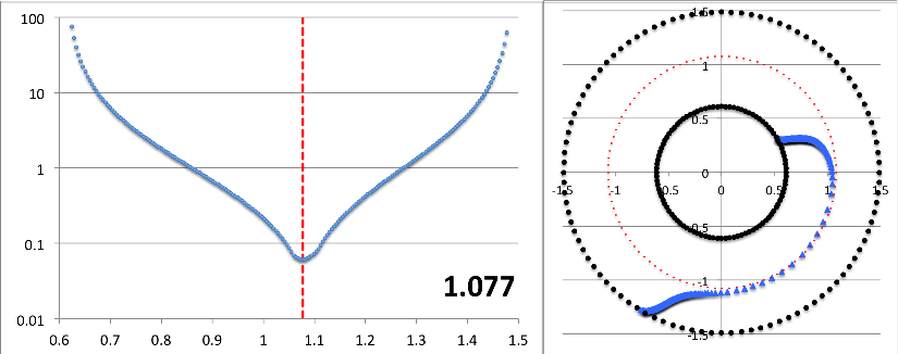
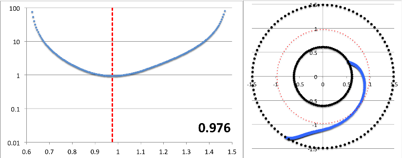
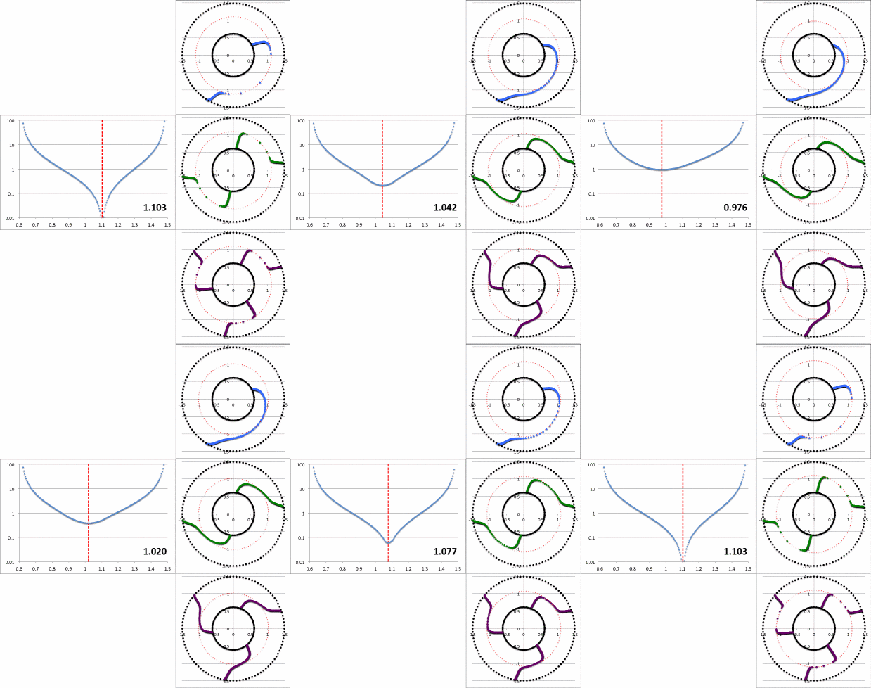
Then, for two separate choices of <math>~r_\mathrm{green}</math> — specifically, 1.05929 and 0.61979 — Table 3 lists values of <math>~f_\mathrm{green}</math> at various radial positions across the HI11 torus. Given values of <math>~f_\mathrm{blue}</math> and <math>~f_\mathrm{green}</math> at each radial position, Table 3 also lists corresponding values of <math>~f_\ln</math>, <math>~D_{1/2}</math>, and <math>~\phi_1</math>. Notice that the values of <math>~[f_\ln]_\mathrm{min}</math> (highlighted in yellow) and <math>~[f_\ln]_\mathrm{max}</math> (highlighted in orange) that are used in the calculation of <math>~D_{1/2}</math> depend on the choice of <math>~r_\mathrm{green}</math>. | |||
<div align="center"> | |||
<table border="1" cellpadding="8" align="center"> | |||
<tr> | |||
<td align="center" colspan="9"> | |||
<font size="+1"><b>Table 3:</b></font><p></p> | |||
Right-hand (green) segment, and total eigenfunction | |||
</td> | |||
</tr> | |||
<tr> | |||
<td align="center" colspan="1" rowspan="2"><math>~r_\mathrm{green}</math></td> | |||
<td align="center" colspan="2">Example Excel Grid Zone</td> | |||
<td align="center" colspan="6">Functions Evaluated<sup>†</sup></td> | |||
<tr> | |||
<td align="center"><math>~N</math></td> | |||
<td align="center"><math>~\varpi</math></td> | |||
<td align="center"><math>~f_\mathrm{green}</math></td> | |||
<td align="center"><math>~f_\mathrm{blue}</math></td> | |||
<td align="center" colspan="2"><math>~f_\ln \equiv \ln(f_\mathrm{green}+f_\mathrm{blue})</math></td> | |||
<td align="center"><math>~D_{1/2}</math></td> | |||
<td align="center"><math>~(\phi_1/\pi)</math></td> | |||
</tr> | |||
<tr> | |||
<td align="center" rowspan="6"> | |||
<math>~$A$102 = 1.05929</math><p> </p> | |||
<p> </p> | |||
<p> </p> | |||
[[File:M02cropped.png|200px|2nd frame of movie]] | |||
</td> | |||
<td align="center">199</td> | |||
<td align="right">1.485605</td> | |||
<td align="right">242.17</td> | |||
<td align="right">0.0</td> | |||
<td align="center">+5.490</td> | |||
<td align="center"> </td> | |||
<td align="center">0.9897</td> | |||
<td align="center">-0.4212</td> | |||
</tr> | |||
<tr> | |||
<td align="center">151</td> | |||
<td align="right">1.274645</td> | |||
<td align="right">1.00000</td> | |||
<td align="right">0.0</td> | |||
<td align="center">0.000</td> | |||
<td align="center"> </td> | |||
<td align="center">0.5750</td> | |||
<td align="center">-0.3695</td> | |||
</tr> | |||
<tr> | |||
<td align="center">112</td> | |||
<td align="right">1.10324</td> | |||
<td align="right">0.073556</td> | |||
<td align="right">0.003475</td> | |||
<td align="center">-2.564</td> | |||
<td align="center"> </td> | |||
<td align="center">0.1662</td> | |||
<td align="center">-0.1868</td> | |||
</tr> | |||
<tr> | |||
<td align="center">106</td> | |||
<td align="right"><font color="red"><b>1.07687</b></font></td> | |||
<td align="right">0.022632</td> | |||
<td align="right">0.038349</td> | |||
<td align="center" bgcolor="yellow">-2.797</td> | |||
<td align="center"><math>~\leftarrow~~[f_\ln]_\mathrm{min}</math></td> | |||
<td align="center">0.0000</td> | |||
<td align="center">0.0000</td> | |||
</tr> | |||
<tr> | |||
<td align="center">103</td> | |||
<td align="right">1.063685</td> | |||
<td align="right">0.004129</td> | |||
<td align="right">0.060897</td> | |||
<td align="center">-2.733</td> | |||
<td align="center"> </td> | |||
<td align="center">0.0871</td> | |||
<td align="center">+0.1068</td> | |||
</tr> | |||
<tr> | |||
<td align="center">1</td> | |||
<td align="right">0.615395</td> | |||
<td align="right">0.0</td> | |||
<td align="right">287.78</td> | |||
<td align="center" bgcolor="orange">+5.662</td> | |||
<td align="center"><math>~\leftarrow~~[f_\ln]_\mathrm{max}</math></td> | |||
<td align="center">1.0000</td> | |||
<td align="center">+0.4220</td> | |||
</tr> | |||
<tr> | |||
<td align="center" colspan="9" bgcolor="purple"> </td> | |||
</tr> | |||
<tr> | |||
<td align="center" rowspan="7"> | |||
<math>~$A$2 = 0.61979</math><p> </p> | |||
<p> </p> | |||
<p> </p> | |||
[[File:M07cropped.png|200px|2nd frame of movie]] | |||
</td> | |||
<td align="center">199</td> | |||
<td align="right">1.485605</td> | |||
<td align="right">566.71</td> | |||
<td align="right">0.0</td> | |||
<td align="center" bgcolor="orange">+6.340</td> | |||
<td align="center"><math>~\leftarrow~~[f_\ln]_\mathrm{max}</math></td> | |||
<td align="center">1.0000</td> | |||
<td align="center">-0.4220</td> | |||
</tr> | |||
<tr> | |||
<td align="center">151</td> | |||
<td align="right">1.274645</td> | |||
<td align="right">3.79829</td> | |||
<td align="right">0.0</td> | |||
<td align="center">+1.335</td> | |||
<td align="center"> </td> | |||
<td align="center">0.4673</td> | |||
<td align="center">-0.3436</td> | |||
</tr> | |||
<tr> | |||
<td align="center">112</td> | |||
<td align="right">1.10324</td> | |||
<td align="right">1.30705</td> | |||
<td align="right">0.003475</td> | |||
<td align="center">+0.270</td> | |||
<td align="center"> </td> | |||
<td align="center">0.2285</td> | |||
<td align="center">-0.2357</td> | |||
</tr> | |||
<tr> | |||
<td align="center">106</td> | |||
<td align="right">1.07687</td> | |||
<td align="right">1.12898</td> | |||
<td align="right">0.038349</td> | |||
<td align="center">+0.155</td> | |||
<td align="center"> </td> | |||
<td align="center">0.1848</td> | |||
<td align="center">-0.2026</td> | |||
</tr> | |||
<tr> | |||
<td align="center">103</td> | |||
<td align="right">1.063685</td> | |||
<td align="right">1.04969</td> | |||
<td align="right">0.060897</td> | |||
<td align="center">+0.105</td> | |||
<td align="center"> </td> | |||
<td align="center">0.1623</td> | |||
<td align="center">-0.1833</td> | |||
</tr> | |||
<tr> | |||
<td align="center">83</td> | |||
<td align="right"><font color="red"><b>0.975785</b></font></td> | |||
<td align="right">0.64322</td> | |||
<td align="right">0.29488</td> | |||
<td align="center" bgcolor="yellow">-0.064</td> | |||
<td align="center"><math>~\leftarrow~~[f_\ln]_\mathrm{min}</math></td> | |||
<td align="center">0.0000</td> | |||
<td align="center">0.0000</td> | |||
</tr> | |||
<tr> | |||
<td align="center">1</td> | |||
<td align="right">0.615395</td> | |||
<td align="right">0.0</td> | |||
<td align="right">287.78</td> | |||
<td align="center">+5.662</td> | |||
<td align="center"> </td> | |||
<td align="center">0.9456</td> | |||
<td align="center">+0.4177</td> | |||
</tr> | |||
<tr> | |||
<td align="left" colspan="9"> | |||
<sup>†</sup>Throughout this table, the phase angle, <math>~\phi_1(\varpi)</math>, has been calculated assuming that <math>~\aleph = 4</math>, and it has been assigned a positive (negative) value if <math>~\varpi</math> is inside (outside) the radial location (identified in red) of the minimum function value, <math>~[f_\ln]_\mathrm{min}</math>. | |||
</td> | |||
</tr> | |||
</table> | |||
</div> | |||
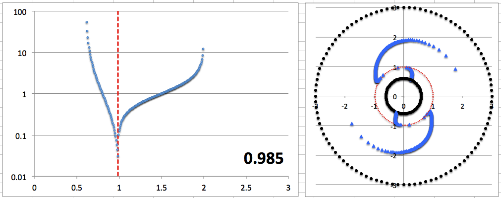
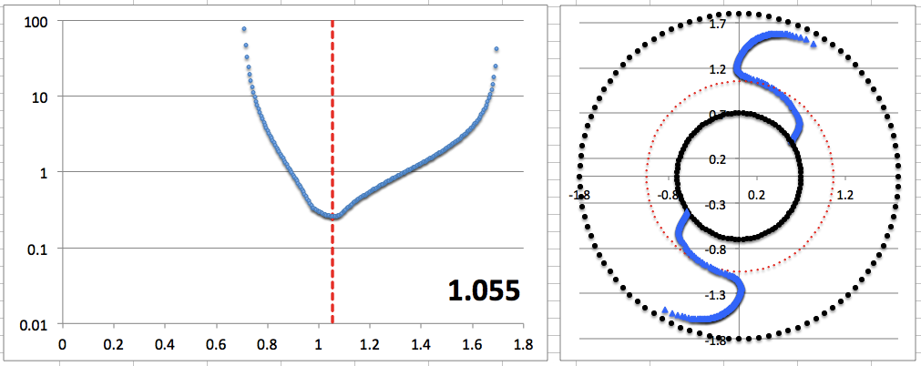
The miniaturized image displayed near the top of the left-most column of Table 3 contains a pair of plots associated with our choice of the parameter, <math>~r_\mathrm{green} = 1.05929</math>: On the left is a semi-log plot of the eigenfunction, <math>~f_\ln</math> versus <math>~\varpi</math> — actually, <math>~f_\mathrm{log10}</math> versus <math>~\varpi</math> — and on the right is a plot in polar coordinates of <math>~\phi_1</math> versus <math>~\varpi</math>, that is, a "constant phase locus" plot. In an analogous manner, the miniaturized image displayed near the bottom of the left-most column of Table 3 contains a semi-log plot of the radial eigenfunction and a polar plot of the "constant phase locus" associated with our choice of the parameter, <math>~r_\mathrm{green} = 0.61979</math>. The pair of plots found in each of these miniaturized images also appear within a single frame of the animation that is displayed in Figure 8, below. Each frame of the animation is stamped with the numerical value corresponding to the radial coordinate, <math>~r_\mathrm{min}</math>, at which the eigenfunction has its minimum (see the red numbers in Table 3). In the case of <math>~r_\mathrm{green} = 1.05929</math>, we find <math>~r_\mathrm{min} = 1.077</math>; and in the case of <math>~r_\mathrm{green} = 0.61979</math>, we find <math>~r_\mathrm{min} = 0.976</math>. | |||
<div align="center"> | |||
<table border="1"> | |||
<tr> | |||
<td align="center" colspan="3"> | |||
<b><font size="+1">Figure 8:</font></b> | |||
Radial and Azimuthal Eigenfunction Comparison | |||
</td> | |||
</tr> | |||
<tr> | |||
<td align="center" colspan="2">'''(a)''' Our Empirically Constructed Function</td> | |||
<td align="center">'''(b)''' Extracted from Figure 16 of [http://adsabs.harvard.edu/abs/2011Ap%26SS.334....1H HI11]</td> | |||
</tr> | |||
<tr> | |||
<td align="center"> | |||
<table border="0" cellpadding="5" align="center"> | |||
<tr> | |||
<td align="center">Specified<p></p><math>~r_\mathrm{green}</math><p></p><hr></td> | |||
<td align="center">Resulting<p></p><math>~r_\mathrm{min}</math><p></p><hr></td> | |||
</tr> | |||
<tr> | |||
<td align="center">1.10324</td> | |||
<td align="center">1.103</td> | |||
</tr> | |||
<tr> | |||
<td align="center">1.05929</td> | |||
<td align="center">1.077</td> | |||
</tr> | |||
<tr> | |||
<td align="center">1.01534</td> | |||
<td align="center">1.059</td> | |||
</tr> | |||
<tr> | |||
<td align="center">0.97139</td> | |||
<td align="center">1.042</td> | |||
</tr> | |||
<tr> | |||
<td align="center">0.88349</td> | |||
<td align="center">1.020</td> | |||
</tr> | |||
<tr> | |||
<td align="center">0.75164</td> | |||
<td align="center">0.998</td> | |||
</tr> | |||
<tr> | |||
<td align="center">0.61979</td> | |||
<td align="center">0.976</td> | |||
</tr> | |||
</table> | |||
</td> | |||
<td align="center"> | |||
[[File:HI11Fig16Animate.gif|350px|Figure 16 from HI11]] | |||
</td> | |||
<td align="center"> | |||
[[File:HI11_Fig16ThreeQuarters.png|400px|Figure 16 from HI11]] | |||
</td> | |||
</tr> | |||
</table> | |||
</div> | |||
{{LSU_WorkInProgress}} | |||
==Attempts to Match P-modes and E-modes== | |||
Based especially on the analysis provided in [http://adsabs.harvard.edu/abs/2011Ap%26SS.334....1H Paper I] and [http://adsabs.harvard.edu/abs/2014Ap%26SS.353..191H Paper II] of the Imamura & Hadley collaboration, the eigenvectors that have drawn our attention thus far can be categorized as J-modes (as discussed, for example, in §3.2.1, Table 1 & Figure 2 of Paper II) or I-modes. Our empirically derived phase function needs to be altered in order to provide reasonable fits to the constant phase loci associated with P-modes and edge-modes (as discussed, for example in §3.2.2, Table2, Figures 3 & 4 of Paper II). We begin by constructing a table of equilibrium parameter values for the typical P- and E-mode models described in Table 2 of [http://adsabs.harvard.edu/abs/2014Ap%26SS.353..191H Paper II]. | |||
===Setup=== | |||
<table border="1" cellpadding="8" align="center"> | |||
<tr> | |||
<td align="center" colspan="10"><font size="+1"><b>Table 4:</b></font> P- and E-mode Model Parameters Highlighted in Paper II | |||
<p></p>[http://adsabs.harvard.edu/abs/2014Ap%26SS.353..191H K. Z. Hadley, P. Fernandez, J. N. Imamura, E. Keever, R. Tumblin, & W. Dumas (2014, ''Astrophysics and Space Science'', 353, 191-222)]</td> | |||
</tr> | |||
<tr> | |||
<td align="center" colspan="6">Extracted from Table 2 or Table 4 of [http://adsabs.harvard.edu/abs/2014Ap%26SS.353..191H Paper II]</td> | |||
<td align="center" colspan="3">Deduced Here</td> | |||
<td align="center" colspan="1">Extracted from Fig. 3 or Fig. 4 of [http://adsabs.harvard.edu/abs/2014Ap%26SS.353..191H Paper II]</td> | |||
</tr> | |||
<tr> | |||
<td align="center">Name</td> | |||
<td align="center"><math>~M_*/M_d</math></td> | |||
<td align="center"><math>~(n, q)</math><sup>†</sup></td> | |||
<td align="center"><math>~R_-/R_+</math></td> | |||
<td align="center"><math>~r_\mathrm{outer} \equiv \frac{R_+}{R_\mathrm{max}}</math></td> | |||
<td align="center"><math>~R_\mathrm{max}</math></td> | |||
<td align="center"><math>~R_+</math></td> | |||
<td align="center"><math>~\epsilon \equiv \frac{R_\mathrm{max}-R_-}{R_\mathrm{max}}</math></td> | |||
<td align="center"><math>~r_- \equiv \frac{R_-}{R_\mathrm{max}}</math></td> | |||
<td align="center">Eigenfunction</td> | |||
</tr> | |||
<tr> | |||
<td align="center">E1</td> | |||
<td align="center"><math>~100</math></td> | |||
<td align="center"><math>~(\tfrac{3}{2}, 2)</math></td> | |||
<td align="center"><math>~0.101</math></td> | |||
<td align="center"><math>~5.52</math></td> | |||
<td align="center"><math>~0.00613</math></td> | |||
<td align="center"><math>~0.0338</math></td> | |||
<td align="center"><math>~0.442</math></td> | |||
<td align="center"><math>~0.558</math></td> | |||
<td align="center"> </td> | |||
</tr> | |||
<tr> | |||
<td align="center">E2</td> | |||
<td align="center"><math>~100</math></td> | |||
<td align="center"><math>~(\tfrac{3}{2}, 2)</math></td> | |||
<td align="center"><math>~0.202</math></td> | |||
<td align="center"><math>~2.99</math></td> | |||
<td align="center"><math>~0.0229</math></td> | |||
<td align="center"><math>~0.0685</math></td> | |||
<td align="center"><math>~0396</math></td> | |||
<td align="center"><math>~0.604</math></td> | |||
<td align="center">[[File:ImamuraPaper2Fig4.png|150px|Model E2]]</td> | |||
</tr> | |||
<tr> | |||
<td align="center">E3</td> | |||
<td align="center"><math>~100</math></td> | |||
<td align="center"><math>~(\tfrac{3}{2}, 2)</math></td> | |||
<td align="center"><math>~0.402</math></td> | |||
<td align="center"><math>~1.74</math></td> | |||
<td align="center"><math>~0.159</math></td> | |||
<td align="center"><math>~0.277</math></td> | |||
<td align="center"><math>~0.301</math></td> | |||
<td align="center"><math>~0.699</math></td> | |||
<td align="center">[[File:ImamuraPaper2Fig4ModelE3.png|150px|Model E3]]</td> | |||
</tr> | |||
<tr> | |||
<td align="center">P1</td> | |||
<td align="center"><math>~100</math></td> | |||
<td align="center"><math>~(\tfrac{3}{2}, 2)</math></td> | |||
<td align="center"><math>~0.452</math></td> | |||
<td align="center"><math>~1.60</math></td> | |||
<td align="center"><math>~0.254</math></td> | |||
<td align="center"><math>~0.406</math></td> | |||
<td align="center"><math>~0.277</math></td> | |||
<td align="center"><math>~0.723</math></td> | |||
<td align="center">[[File:ImamuraPaper2Fig3ModelP1.png|150px|Model P1]]</td> | |||
</tr> | |||
<tr> | |||
<td align="center">P2</td> | |||
<td align="center"><math>~100</math></td> | |||
<td align="center"><math>~(\tfrac{3}{2}, 2)</math></td> | |||
<td align="center"><math>~0.500</math></td> | |||
<td align="center"><math>~1.49</math></td> | |||
<td align="center"><math>~0.403</math></td> | |||
<td align="center"><math>~0.600</math></td> | |||
<td align="center"><math>~0.255</math></td> | |||
<td align="center"><math>~0.745</math></td> | |||
<td align="center">[[File:ImamuraPaper2Fig3ModelP2.png|150px|Model P2]]</td> | |||
</tr> | |||
<tr> | |||
<td align="center">P3</td> | |||
<td align="center"><math>~100</math></td> | |||
<td align="center"><math>~(\tfrac{3}{2}, 2)</math></td> | |||
<td align="center"><math>~0.600</math></td> | |||
<td align="center"><math>~1.33</math></td> | |||
<td align="center"><math>~1.09</math></td> | |||
<td align="center"><math>~1.450</math></td> | |||
<td align="center"><math>~0.202</math></td> | |||
<td align="center"><math>~0.798</math></td> | |||
<td align="center"> </td> | |||
</tr> | |||
<tr> | |||
<td align="center">P4</td> | |||
<td align="center"><math>~100</math></td> | |||
<td align="center"><math>~(\tfrac{3}{2}, 2)</math></td> | |||
<td align="center"><math>~0.700</math></td> | |||
<td align="center"><math>~1.21</math></td> | |||
<td align="center"><math>~3.37</math></td> | |||
<td align="center"><math>~4.078</math></td> | |||
<td align="center"><math>~0.153</math></td> | |||
<td align="center"><math>~0.847</math></td> | |||
<td align="center"> </td> | |||
</tr> | |||
<tr> | |||
<td align="left" colspan="10"><sup>†</sup>In all three papers from the [[#See_Also|Imamura & Hadley collaboration]], <math>~q = 2</math> means, "[[User:Tohline/AxisymmetricConfigurations/SolutionStrategies#Simple_Rotation_Profile_and_Centrifugal_Potential|uniform specific angular momentum]]."</td> | |||
</tr> | |||
</table> | |||
[[User:Tohline/Appendix/Ramblings/To_Hadley_and_Imamura#Recognition_.233|As in our separate summary discussion]], our two-piece radial eigenfunction is defined by the expressions, | |||
<div align="center"> | |||
<table border="0" cellpadding="5" align="center"> | |||
<tr> | |||
<td align="center" bgcolor="blue"> </td> | |||
<td align="right"> | |||
<math>~f_\mathrm{blue}(\varpi) </math> | |||
</td> | |||
<td align="center"> | |||
<math>~=</math> | |||
</td> | |||
<td align="left"> | |||
<math>~\biggl( \frac{r_\mathrm{blue} - \varpi}{\varpi - r_-} \biggr)^{p} | |||
</math> | |||
</td> | |||
<td align="center"> | |||
for | |||
</td> | |||
<td align="left"> | |||
<math>r_- < \varpi < r_\mathrm{blue} </math> | |||
… | |||
<math>~\biggl[ f_\mathrm{blue}(\varpi) = 0</math> otherwise<math>~\biggr]</math>, | |||
</td> | |||
</tr> | |||
</table> | |||
</div> | |||
and, | |||
<div align="center"> | |||
<table border="0" cellpadding="5" align="center"> | |||
<tr> | |||
<td align="center" bgcolor="green"> </td> | |||
<td align="right"> | |||
<math>~f_\mathrm{green}(\varpi) </math> | |||
</td> | |||
<td align="center"> | |||
<math>~=</math> | |||
</td> | |||
<td align="left"> | |||
<math>~\biggl( \frac{r_\mathrm{green} - \varpi}{\varpi - r_+} \biggr)^{p} | |||
</math> | |||
</td> | |||
<td align="center"> | |||
for | |||
</td> | |||
<td align="left"> | |||
<math>r_\mathrm{green} < \varpi < r_+ </math> | |||
… | |||
<math>~\biggl[ f_\mathrm{green}(\varpi) = 0</math> otherwise<math>~\biggr]</math>, | |||
</td> | |||
</tr> | |||
</table> | |||
</div> | |||
where, <math>~r_\mathrm{mid}|_\mathrm{green} \le r_\mathrm{mid}|_\mathrm{blue}</math>. The expression that we are currently using for the radial eigenfunction is a sum of these two pieces, that is, | |||
<div align="center"> | |||
<table border="1" cellpadding="8" align="center"> | |||
<tr><td align="center"> | |||
<table border="0" cellpadding="5" align="center"> | |||
<tr> | |||
<td align="right"> | |||
<math>~f_2(\varpi)</math> | |||
</td> | |||
<td align="center"> | |||
<math>~=</math> | |||
</td> | |||
<td align="left"> | |||
<math>~f_\mathrm{green}(\varpi) + f_\mathrm{blue}(\varpi) \, . | |||
</math> | |||
</td> | |||
</tr> | |||
</table> | |||
</td></tr> | |||
</table> | |||
</div> | |||
Over the inner ("blue") region of the torus, we will continue to use the phase-function prescription that has been described [[User:Tohline/Appendix/Ramblings/To_Hadley_and_Imamura#Constant_Phase_Loci|in our separate summary discussion]], namely, | |||
<div align="center"> | |||
<table border="0" cellpadding="8" align="center"> | |||
<tr><td align="center"> | |||
<table border="0" cellpadding="5" align="center"> | |||
<tr> | |||
<td align="center" bgcolor="blue"> </td> | |||
<td align="right"> | |||
<math>~m\phi_\mathrm{blue}</math> | |||
</td> | |||
<td align="center"> | |||
<math>~=</math> | |||
</td> | |||
<td align="left"> | |||
<math>~\pm \tan^{-1}[\aleph_m \cdot D_{1/2}(\varpi)] </math> | |||
</td> | |||
<td align="center"> | |||
for | |||
</td> | |||
<td align="left"> | |||
<math>r_- < \varpi < r_\mathrm{min} \, ,</math> | |||
</td> | |||
</tr> | |||
</table> | |||
</td></tr> | |||
</table> | |||
</div> | |||
where, <math>~\aleph_m</math> is a constant, | |||
<div align="center"> | |||
<table border="0" cellpadding="5" align="center"> | |||
<tr> | |||
<td align="right"> | |||
<math>~D_{1/2}(\varpi)</math> | |||
</td> | |||
<td align="center"> | |||
<math>~\equiv</math> | |||
</td> | |||
<td align="left"> | |||
<math>~\biggl[ \frac{f_\ln(\varpi) - [f_\ln]_\mathrm{min}}{[f_\ln]_\mathrm{max} - [f_\ln]_\mathrm{min}} \biggr]^{1/2} \, ,</math> | |||
</td> | |||
</tr> | |||
<tr> | |||
<td align="right"> | |||
<math>~f_\ln(\varpi)</math> | |||
</td> | |||
<td align="center"> | |||
<math>~\equiv</math> | |||
</td> | |||
<td align="left"> | |||
<math>~\ln[ f_1(\varpi)] \, .</math> | |||
</td> | |||
</tr> | |||
</table> | |||
</div> | |||
and, <math>~r_\mathrm{min}</math> is the radial location of the minimum of the radial eigenfunction, <math>~f_\ln</math>. Over the outer ("green") region of the torus, however, we now adopt a different prescription for the phase function, namely, | |||
<div align="center"> | |||
<table border="0" cellpadding="8" align="center"> | |||
<tr><td align="center"> | |||
<table border="0" cellpadding="5" align="center"> | |||
<tr> | |||
<td align="center" bgcolor="green"> </td> | |||
<td align="right"> | |||
<math>~m\phi_\mathrm{green}</math> | |||
</td> | |||
<td align="center"> | |||
<math>~=</math> | |||
</td> | |||
<td align="left"> | |||
<math>~\frac{1}{A_0}\cdot \sin[\aleph_m \cdot D_{1/2}(\varpi)] </math> | |||
</td> | |||
<td align="center"> | |||
for | |||
</td> | |||
<td align="left"> | |||
<math>r_\mathrm{min} < \varpi < r_+ \, ,</math> | |||
</td> | |||
</tr> | |||
</table> | |||
</td></tr> | |||
</table> | |||
</div> | |||
where, <math>~A_0</math> is a constant. | |||
===Application to Specific Models=== | |||
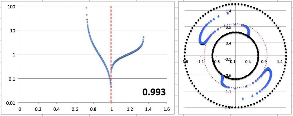
In what follows, we pick a model from Table 4, and extract from that model the locations of the inner and outer radii of the torus, namely, <math>~r_-</math> and <math>~r_\mathrm{outer}</math>. Then, in an effort to construct an eigenvector that matches the behavior shown in the corresponding Paper II plots (as reprinted, here, in the last column of our Table 4) over the innermost region of the configuration — that is, the region around the innermost and most prominent minimum of the radial eigenfunction — we assign a value to <math>~r_\mathrm{blue}</math> that roughly corresponds to the radial location of the first (innermost) minimum, and we assign a value to <math>~r_+</math> that roughly corresponds to the radial location of the second minimum. We set <math>~m = 2</math> for each model, because, following [http://adsabs.harvard.edu/abs/2014Ap%26SS.353..191H Hadley et al. (2014)], we are focusing only on unstable P- and E-modes having "bar-like" structures; and, [[#Specific_Application_to_HI11.27s_Figure_16|as above]], when descritizing each model within Excel, we set, | |||
<div align="center"> | |||
<table border="0" cellpadding="5" align="center"> | |||
<tr> | |||
<td align="right"> | |||
<math>~\delta r</math> | |||
</td> | |||
<td align="center"> | |||
<math>~=</math> | |||
</td> | |||
<td align="left"> | |||
<math>~\frac{r_+ - r_-}{200} </math> | |||
</td> | |||
</tr> | |||
<tr> | |||
<td align="right"> | |||
<math>~$A$N</math> | |||
</td> | |||
<td align="center"> | |||
<math>~=</math> | |||
</td> | |||
<td align="left"> | |||
<math>~r_- + N \delta r \, .</math> | |||
</td> | |||
</tr> | |||
</table> | |||
</div> | |||
Then, for each model, we adjusted the values of five free parameters until a reasonably good fit to both the published radial eigenfunction and "constant phase locus" was obtained over the innermost region of the model. The five adjustable parameters are: <math>~p_\mathrm{blue}, ~r_\mathrm{green}, ~p_\mathrm{green}, ~\aleph_2,</math> and <math>~A_0</math>. | |||
<div align="center" id="Table5"> | |||
<table border="1" align="center" cellpadding="5" width="75%"> | |||
<tr><td align="center" colspan="5" bgcolor="yellow"><font size="+1"><b>Table 5:</b></font> Model E2<sup>‡</sup></td></tr> | |||
<tr> | |||
<td align="center" colspan="4" bgcolor="white"><font size="+1"><b>Model Parameters</b></font></td> | |||
<td align="center" colspan="1" rowspan="1" bgcolor="white">Results from [http://adsabs.harvard.edu/abs/2014Ap%26SS.353..191H Paper II (Hadley et al. 2014)] Simulation</td> | |||
</tr> | |||
<tr> | |||
<td align="center"><math>~r_-</math></td> | |||
<td align="center"><math>~r_+</math></td> | |||
<td align="center"><math>~r_\mathrm{outer}</math></td> | |||
<td align="center"><math>~\delta r</math></td> | |||
<td align="center" colspan="1" rowspan="6"> | |||
[[File:ImamuraPaper2Fig4.png|400px|right|Figure 4b from Paper II]] | |||
</td> | |||
</tr> | |||
<tr> | |||
<td align="center"><math>~0.60</math></td> | |||
<td align="center"><math>~2.0</math></td> | |||
<td align="center"><math>~3.0</math></td> | |||
<td align="center"><math>~0.007</math></td> | |||
</tr> | |||
<tr> | |||
<td bgcolor="gray" colspan="4"> </td> | |||
</tr> | |||
<tr> | |||
<td align="center"><math>~r_\mathrm{blue}</math></td> | |||
<td align="center" bgcolor="lightblue"><math>~p_\mathrm{blue}</math></td> | |||
<td align="center" bgcolor="lightblue"><math>~r_\mathrm{green}</math></td> | |||
<td align="center" bgcolor="lightblue"><math>~p_\mathrm{green}</math></td> | |||
</tr> | |||
<tr> | |||
<td align="center"><math>~$A$68 = 1.006</math></td> | |||
<td align="center"><math>~1.2</math></td> | |||
<td align="center"><math>~$A$65 = 0.985</math></td> | |||
<td align="center"><math>~0.50</math></td> | |||
</tr> | |||
<tr> | |||
<td bgcolor="gray" colspan="4"> </td> | |||
</tr> | |||
<tr> | |||
<td align="center"><math>~r_\mathrm{min}</math></td> | |||
<td align="center"><math>~[f_\ln]_\mathrm{min}</math></td> | |||
<td align="center" colspan="2"><math>~[f_\ln]_\mathrm{max}</math></td> | |||
<td align="center" colspan="1" bgcolor="white">Our Empirically Constructed Eigenvector</td> | |||
</tr> | |||
<tr> | |||
<td align="center"><math>~$A$65 = 0.985</math></td> | |||
<td align="center"><math>~-3.49047</math></td> | |||
<td align="center" colspan="2"><math>~\ln[f_2($A$1)]=+4.85166</math></td> | |||
<td align="center" colspan="1" rowspan="5"> | |||
[[File:ImamuraPaper2MyE2mirror.png|380px|right|Empirically constructed E2]] | |||
</td> | |||
</tr> | |||
<tr> | |||
<td bgcolor="gray" colspan="4"> </td> | |||
</tr> | |||
<tr> | |||
<td align="center"><math>~m</math></td> | |||
<td align="center" bgcolor="lightblue"><math>~\aleph_2</math></td> | |||
<td align="center" bgcolor="lightblue"><math>~A_0</math></td> | |||
<td align="center"><math>~\phi_0</math></td> | |||
</tr> | |||
<tr> | |||
<td align="center"><math>~2</math></td> | |||
<td align="center"><math>~\pi</math></td> | |||
<td align="center"><math>~0.25</math></td> | |||
<td align="center"><math>~\tfrac{9\pi}{16}</math></td> | |||
</tr> | |||
<tr> | |||
<td bgcolor="gray" colspan="4"> </td> | |||
</tr> | |||
<tr> | |||
<td align="left" colspan="5"> | |||
<sup>‡</sup>Note the following: | |||
* When the Paper II radial eigenfunction possesses more than one local minimum — and, in tandem, the Paper II phase function swings through more than <math>~2\pi</math> radians — we have set the parameter, <math>~r_+</math>, to a value less than <math>~r_\mathrm{outer}</math> because our empirically constructed eigenfunction is only designed to accommodate a single (the innermost) function minimum. | |||
* Our empirical model's 5 adjustable free parameters are highlighted in blue. | |||
* Before plotting our empirically constructed phase function, the tabulated phase shift, <math>~\phi_0</math>, has been added to both <math>~\phi_\mathrm{blue}</math> and <math>~\phi_\mathrm{green}</math> in an effort to match the overall orientation of the "constant phase locus" published in Paper II. (This is not considered to be an adjustable free parameter.) | |||
</td> | |||
</tr> | |||
</table> | |||
</div> | |||
<p></p> | |||
<p></p> | |||
<div align="center" id="Table6"> | |||
<table border="1" align="center" cellpadding="5" width="75%"> | |||
<tr><td align="center" colspan="5" bgcolor="yellow"><font size="+1"><b>Table 6:</b></font> Model E3<sup>‡</sup></td></tr> | |||
<tr> | |||
<td align="center" colspan="4" bgcolor="white"><font size="+1"><b>Model Parameters</b></font></td> | |||
<td align="center" colspan="1" rowspan="1" bgcolor="white">Results from [http://adsabs.harvard.edu/abs/2014Ap%26SS.353..191H Paper II (Hadley et al. 2014)] Simulation</td> | |||
</tr> | |||
<tr> | |||
<td align="center"><math>~r_-</math></td> | |||
<td align="center"><math>~r_+</math></td> | |||
<td align="center"><math>~r_\mathrm{outer}</math></td> | |||
<td align="center"><math>~\delta r</math></td> | |||
<td align="center" colspan="1" rowspan="6"> | |||
[[File:ImamuraPaper2Fig4ModelE3.png|400px|right|Figure 4a from Paper II]] | |||
</td> | |||
</tr> | |||
<tr> | |||
<td align="center"><math>~0.7</math></td> | |||
<td align="center"><math>~1.7</math></td> | |||
<td align="center"><math>~1.74</math></td> | |||
<td align="center"><math>~0.005</math></td> | |||
</tr> | |||
<tr> | |||
<td bgcolor="gray" colspan="4"> </td> | |||
</tr> | |||
<tr> | |||
<td align="center" bgcolor="white"><math>~r_\mathrm{blue}</math></td> | |||
<td align="center" bgcolor="lightblue"><math>~p_\mathrm{blue}</math></td> | |||
<td align="center" bgcolor="lightblue"><math>~r_\mathrm{green}</math></td> | |||
<td align="center" bgcolor="lightblue"><math>~p_\mathrm{green}</math></td> | |||
</tr> | |||
<tr> | |||
<td align="center"><math>~$A$77 = 1.085</math></td> | |||
<td align="center"><math>~1.2</math></td> | |||
<td align="center"><math>~$A$55 = 0.975</math></td> | |||
<td align="center"><math>~0.75</math></td> | |||
</tr> | |||
<tr> | |||
<td bgcolor="gray" colspan="4"> </td> | |||
</tr> | |||
<tr> | |||
<td align="center"><math>~r_\mathrm{min}</math></td> | |||
<td align="center"><math>~[f_\ln]_\mathrm{min}</math></td> | |||
<td align="center" colspan="2"><math>~[f_\ln]_\mathrm{max}</math></td> | |||
<td align="center" colspan="1" bgcolor="white">Our Empirically Constructed Eigenvector</td> | |||
</tr> | |||
<tr> | |||
<td align="center"><math>~$A$71 = 1.055</math></td> | |||
<td align="center"><math>~-1.34494</math></td> | |||
<td align="center" colspan="2"><math>~\ln[f_2($A$1)]=+5.19688</math></td> | |||
<td align="center" colspan="1" rowspan="5"> | |||
[[File:ImamuraPaper2MyE3mirror.png|380px|right|Empirically constructed E3]] | |||
</td> | |||
</tr> | |||
<tr> | |||
<td bgcolor="gray" colspan="4"> </td> | |||
</tr> | |||
<tr> | |||
<td align="center"><math>~m</math></td> | |||
<td align="center" bgcolor="lightblue"><math>~\aleph_2</math></td> | |||
<td align="center" bgcolor="lightblue"><math>~A_0</math></td> | |||
<td align="center"><math>~\phi_0</math></td> | |||
</tr> | |||
<tr> | |||
<td align="center"><math>~2</math></td> | |||
<td align="center"><math>~\tfrac{11 \pi}{8}</math></td> | |||
<td align="center"><math>~3.0</math></td> | |||
<td align="center"><math>~\tfrac{2\pi}{5}</math></td> | |||
</tr> | |||
<tr> | |||
<td bgcolor="gray" colspan="4"> </td> | |||
</tr> | |||
<tr> | |||
<td align="left" colspan="5"> | |||
<sup>‡</sup>Note the following: | |||
* When the Paper II radial eigenfunction possesses more than one local minimum — and, in tandem, the Paper II phase function swings through more than <math>~2\pi</math> radians — we have set the parameter, <math>~r_+</math>, to a value less than <math>~r_\mathrm{outer}</math> because our empirically constructed eigenfunction is only designed to accommodate a single (the innermost) function minimum. | |||
* Our empirical model's 5 adjustable free parameters are highlighted in blue. | |||
* The undesirable kink that appears in our empirically constructed radial eigenfunction (to the left of the function minimum) arises because the exponent, <math>~p_\mathrm{green}</math>, is a fraction that is less than unity. | |||
* Before plotting our empirically constructed phase function, the tabulated phase shift, <math>~\phi_0</math>, has been added to both <math>~\phi_\mathrm{blue}</math> and <math>~\phi_\mathrm{green}</math> in an effort to match the overall orientation of the "constant phase locus" published in Paper II. (This is not considered to be an adjustable free parameter.) | |||
</td> | |||
</tr> | |||
</table> | |||
</div> | |||
<!-- COMMENT OUT OLD TABLE 5 | |||
<table border="1" align="center" cellpadding="5"> | |||
<tr><td align="center" colspan="14"><font size="+1"><b>Table 5:</b></font> Empirical Fits<sup>‡</sup></td></tr> | |||
<tr> | |||
<td align="center">Name</td> | |||
<td align="center"><math>~r_-</math></td> | |||
<td align="center"><math>~r_+</math></td> | |||
<td align="center"><math>~\delta r</math></td> | |||
<td align="center"><math>~r_\mathrm{blue}</math></td> | |||
<td align="center"><math>~p_\mathrm{blue}</math></td> | |||
<td align="center"><math>~r_\mathrm{green}</math></td> | |||
<td align="center"><math>~p_\mathrm{green}</math></td> | |||
<td align="center"><math>~r_\mathrm{min}</math></td> | |||
<td align="center"><math>~[f_\ln]_\mathrm{min}</math></td> | |||
<td align="center"><math>~[f_\ln]_\mathrm{max}=\ln[f_2($A$1)]</math></td> | |||
<td align="center"><math>~m</math></td> | |||
<td align="center"><math>~\aleph_2</math></td> | |||
<td align="center"><math>~A_0</math></td> | |||
</tr> | |||
<tr> | |||
<td align="center">E3</td> | |||
<td align="center"><math>~0.7</math></td> | |||
<td align="center"><math>~1.7</math></td> | |||
<td align="center"><math>~0.005</math></td> | |||
<td align="center"><math>~$A$77 = 1.085</math></td> | |||
<td align="center"><math>~1.2</math></td> | |||
<td align="center"><math>~$A$55 = 0.975</math></td> | |||
<td align="center"><math>~0.75</math></td> | |||
<td align="center"><math>~$A$71 = 1.055</math></td> | |||
<td align="center"><math>~-1.34494</math></td> | |||
<td align="center"><math>~+5.19688</math></td> | |||
<td align="center"><math>~2</math></td> | |||
<td align="center"><math>~\tfrac{11 \pi}{8}</math></td> | |||
<td align="center"><math>~3.0</math></td> | |||
</tr> | |||
<tr> | |||
<td align="center" colspan="14"> | |||
[[File:ImamuraPaper2Fig4ModelE3.png|400px|Model E3]]<p></p> | |||
[[File:ImamuraPaper2MyE3.png|400px|My E3]] | |||
</td> | |||
</tr> | |||
<tr> | |||
<td align="left" colspan="14"> | |||
<sup>‡</sup>Note the following: | |||
* When the Paper II radial eigenfunction possesses more than one local minimum — and, in tandem, the Paper II phase function swings through more than <math>~2\pi</math> radians — we have set the parameter, <math>~r_+</math>, to a value less than <math>~r_\mathrm{outer}</math> because our empirically constructed eigenfunction is only designed to accommodate a single (the innermost) function minimum. | |||
* The undesirable kink that appears in our empirically constructed radial eigenfunction, to the left of the function minimum, arises because the exponent, <math>~p_\mathrm{green}</math>, is a fraction that is less than unity. | |||
</td> | |||
</tr> | |||
</table> | |||
END COMMENTING OUT OLD TABLE 5 --> | |||
<p></p> | |||
<p></p> | |||
<div align="center" id="Table7"> | |||
<table border="1" align="center" cellpadding="5" width="75%"> | |||
<tr><td align="center" colspan="5" bgcolor="yellow"><font size="+1"><b>Table 7:</b></font> Model P1<sup>‡</sup></td></tr> | |||
<tr> | |||
<td align="center" colspan="4" bgcolor="white"><font size="+1"><b>Model Parameters</b></font></td> | |||
<td align="center" colspan="1" rowspan="1" bgcolor="white">Results from [http://adsabs.harvard.edu/abs/2014Ap%26SS.353..191H Paper II (Hadley et al. 2014)] Simulation</td> | |||
</tr> | |||
<tr> | |||
<td align="center"><math>~r_-</math></td> | |||
<td align="center"><math>~r_+</math></td> | |||
<td align="center"><math>~r_\mathrm{outer}</math></td> | |||
<td align="center"><math>~\delta r</math></td> | |||
<td align="center" colspan="1" rowspan="6"> | |||
[[File:ImamuraPaper2Fig3ModelP1.png|400px|right|Figure 3d from Paper II]] | |||
</td> | |||
</tr> | |||
<tr> | |||
<td align="center"><math>~0.723</math></td> | |||
<td align="center"><math>~1.35</math></td> | |||
<td align="center"><math>~1.6</math></td> | |||
<td align="center"><math>~0.003135</math></td> | |||
</tr> | |||
<tr> | |||
<td bgcolor="gray" colspan="4"> </td> | |||
</tr> | |||
<tr> | |||
<td align="center" bgcolor="white"><math>~r_\mathrm{blue}</math></td> | |||
<td align="center" bgcolor="lightblue"><math>~p_\mathrm{blue}</math></td> | |||
<td align="center" bgcolor="lightblue"><math>~r_\mathrm{green}</math></td> | |||
<td align="center" bgcolor="lightblue"><math>~p_\mathrm{green}</math></td> | |||
</tr> | |||
<tr> | |||
<td align="center"><math>~$A$100 = 1.00515</math></td> | |||
<td align="center"><math>~1.0</math></td> | |||
<td align="center"><math>~$A$96 = 0.99261</math></td> | |||
<td align="center"><math>~0.35</math></td> | |||
</tr> | |||
<tr> | |||
<td bgcolor="gray" colspan="4"> </td> | |||
</tr> | |||
<tr> | |||
<td align="center"><math>~r_\mathrm{min}</math></td> | |||
<td align="center"><math>~[f_\ln]_\mathrm{min}</math></td> | |||
<td align="center" colspan="2"><math>~[f_\ln]_\mathrm{max}</math></td> | |||
<td align="center" colspan="1" bgcolor="white">Our Empirically Constructed Eigenvector</td> | |||
</tr> | |||
<tr> | |||
<td align="center"><math>~$A$96 = 0.99261</math></td> | |||
<td align="center"><math>~-3.06805</math></td> | |||
<td align="center" colspan="2"><math>~\ln[f_2($A$1)]=+4.48864</math></td> | |||
<td align="center" colspan="1" rowspan="5"> | |||
[[File:ImamuraPaper2MyP1better.png|380px|right|Empirically constructed P1]] | |||
</td> | |||
</tr> | |||
<tr> | |||
<td bgcolor="gray" colspan="4"> </td> | |||
</tr> | |||
<tr> | |||
<td align="center"><math>~m</math></td> | |||
<td align="center" bgcolor="lightblue"><math>~\aleph_2</math></td> | |||
<td align="center" bgcolor="lightblue"><math>~A_0</math></td> | |||
<td align="center"><math>~\phi_0</math></td> | |||
</tr> | |||
<tr> | |||
<td align="center"><math>~2</math></td> | |||
<td align="center"><math>~2.55</math></td> | |||
<td align="center"><math>~0.094</math></td> | |||
<td align="center"><math>~\tfrac{\pi}{2}</math></td> | |||
</tr> | |||
<tr> | |||
<td bgcolor="gray" colspan="4"> </td> | |||
</tr> | |||
<tr> | |||
<td align="left" colspan="5"> | |||
<sup>‡</sup>Note the following: | |||
* When the Paper II radial eigenfunction possesses more than one local minimum — and, usually in tandem, the Paper II phase function swings through more than <math>~2\pi</math> radians — we have set the parameter, <math>~r_+</math>, to a value less than <math>~r_\mathrm{outer}</math> because our empirically constructed eigenfunction is only designed to accommodate a single (the innermost) function minimum. | |||
* Our empirical model's 5 adjustable free parameters are highlighted in blue. | |||
* Before plotting our empirically constructed phase function, the tabulated phase shift, <math>~\phi_0</math>, has been added to both <math>~\phi_\mathrm{blue}</math> and <math>~\phi_\mathrm{green}</math> in an effort to match the overall orientation of the "constant phase locus" published in Paper II. (This is not considered to be an adjustable free parameter.) | |||
</td> | |||
</tr> | |||
</table> | |||
</div> | |||
=See Also= | =See Also= | ||
* Imamura & Hadley collaboration: | |||
** <font color="red"><b>Paper I</b></font>: [http://adsabs.harvard.edu/abs/2011Ap%26SS.334....1H K. Hadley & J. N. Imamura (2011, ''Astrophysics and Space Science'', 334, 1-26)], "Nonaxisymmetric instabilities in self-gravitating disks. I. Toroids" — In this paper, Hadley & Imamura perform linear stability analyses on fully self-gravitating toroids; that is, there is no central point-like stellar object and, hence, <math>~M_*/M_d = 0.0</math>. | |||
** <font color="red"><b>Paper II</b></font>: [http://adsabs.harvard.edu/abs/2014Ap%26SS.353..191H K. Z. Hadley, P. Fernandez, J. N. Imamura, E. Keever, R. Tumblin, & W. Dumas (2014, ''Astrophysics and Space Science'', 353, 191-222)], "Nonaxisymmetric instabilities in self-gravitating disks. II. Linear and quasi-linear analyses" — In this paper, the Imamura & Hadley collaboration performs "an extensive study of nonaxisymmetric global instabilities in thick, self-gravitating star-disk systems creating a large catalog of star/disk systems … for star masses of <math>~0.0 \le M_*/M_d \le 10^3</math> and inner to outer edge aspect ratios of <math>~0.1 < r_-/r_+ < 0.75</math>." | |||
** <font color="red"><b>Paper III</b></font>: [http://adsabs.harvard.edu/abs/2015Ap%26SS.359...10H K. Z. Hadley, W. Dumas, J. N. Imamura, E. Keever, & R. Tumblin (2015, ''Astrophysics and Space Science'', 359, article id. 10, 23 pp.)], "Nonaxisymmetric instabilities in self-gravitating disks. III. Angular momentum transport" — In this paper, the Imamura & Hadley collaboration carries out nonlinear simulations of nonaxisymmetric instabilities found in self-gravitating star/disk systems and compares these results with the linear and quasi-linear modeling results presented in Papers I and II. | |||
{{LSU_HBook_footer}} | {{LSU_HBook_footer}} | ||
Latest revision as of 20:56, 24 May 2016
Analyzing Azimuthal Distortions
[Comment by J. E. Tohline on 24 May 2016] This chapter contains a set of technical notes and accompanying discussion that I put together several months ago as I was trying to gain a foundational understanding of the results of a large study of instabilities in self-gravitating tori published by the Imamura & Hadley collaboration. I have come to appreciate that some of the logic and interpretation of published results that are presented, below, has serious flaws. Therefore, anyone reading this should be quite cautious in deciding what subsections provide useful insight. I have written a separate chapter titled, "Characteristics of Unstable Eigenvectors in Self-Gravitating Tori," that contains a much more trustworthy analysis of this very interesting problem.
Material that appears after this point in our presentation is under development and therefore
may contain incorrect mathematical equations and/or physical misinterpretations.
| Go Home |

|
|---|
| | Tiled Menu | Tables of Content | Banner Video | Tohline Home Page | |
In what follows, we will draw heavily from three publications: (1) J. E. Tohline & I. Hachisu (1990, ApJ, 361, 394-407) — hereafter, TH90 — (2) J. W. Woodward, J. E. Tohline, & I. Hachisu (1994, ApJ, 420, 247-267) — hereafter, WTH94 — and (3) K. Hadley & J. N. Imamura (2011, Astrophysics and Space Science, 334, 1) — hereafter, HI11.
Adopted Notation
Beginning with equation (2) of TH90 but ignoring variations in the vertical coordinate direction, the mass density is given by the expression,
|
<math>~\rho</math> |
<math>~=</math> |
<math>~\rho_0 \biggl[ 1 + f(\varpi)e^{-i(\omega t - m\phi)} \biggr] \, ,</math> |
where it is understood that <math>~\rho_0</math>, which defines the structure of the initial axisymmetric equilibrium configuration, is generally a function of the cylindrical radial coordinate, <math>~\varpi</math>.
Using the subscript, <math>~m</math>, to identify the time-invariant coefficients and functions that characterize the intrinsic eigenvector of each azimuthal eigen-mode, and acknowledging that the associated eigenfrequency will in general be imaginary, that is,
|
<math>~\omega_m</math> |
<math>~=</math> |
<math>~\omega_R + i\omega_I \, ,</math> |
we expect each unstable mode to display the following behavior:
|
<math>~\biggl[ \frac{\rho}{\rho_0} - 1 \biggr]</math> |
<math>~=</math> |
<math>~f_m(\varpi)e^{-i[\omega_R t + i \omega_I t - m\phi_m(\varpi)]} </math> |
|
|
<math>~=</math> |
<math>~\biggl\{ f_m(\varpi)e^{-im\phi_m(\varpi)}\biggr\} e^{-i\omega_R t } \cdot e^{\omega_I t} </math> |
|
|
<math>~=</math> |
<math>~\biggl\{ f_m(\varpi)e^{-i[\omega_R t + m\phi_m(\varpi)]} \biggr\} e^{\omega_I t} \, .</math> |
Adopting Kojima's (1986) notation, that is, defining,
|
<math>~y_1 \equiv \frac{\omega_R}{\Omega_0} - m</math> |
and |
<math>~y_2 \equiv \frac{\omega_I}{\Omega_0} \, ,</math> |
the eigenvector's behavior can furthermore be described by the expression,
|
<math>~\biggl[ \frac{\rho}{\rho_0} - 1 \biggr]</math> |
<math>~=</math> |
<math>~\biggl\{ f_m(\varpi)e^{-i[(y_1+m) (\Omega_0 t) + m\phi_m(\varpi)]} \biggr\} e^{y_2 (\Omega_0 t)} </math> |
|
|
<math>~=</math> |
<math>~\biggl\{ f_m(\varpi)e^{-im[(y_1/m+1) (\Omega_0 t) + \phi_m(\varpi)]} \biggr\} e^{y_2 (\Omega_0 t)} \, .</math> |
Note that, as viewed from a frame of reference that is rotating with the mode pattern frequency,
<math>\Omega_p \equiv \frac{\omega_R}{m} = \Omega_0\biggl(\frac{y_1}{m}+1\biggr) \, ,</math>
we should find an eigenvector of the form,
|
<math>~\biggl[ \frac{\delta\rho}{\rho_0}\biggr]_\mathrm{rot} \equiv \biggl[ \frac{\rho}{\rho_0} - 1 \biggr]e^{im\Omega_p t}</math> |
<math>~=</math> |
<math>~\biggl\{ f_m(\varpi)e^{-im[\phi_m(\varpi)]} \biggr\} e^{y_2 (\Omega_0 t)} \, ,</math> |
whose relative amplitude — with a radial structure as specified inside the curly braces — is undergoing a uniform exponential growth but is otherwise unchanging.
Drawing from figure 2 of WTH94, our Figure 1, immediately below, illustrates how the behavior of each factor in this expression can reveal itself during a numerical simulation that follows the time-evolutionary development of an unstable, nonaxisymmetric eigenmode. The initial model for this depicted evolution (model O3 from Table 1 of WTH94) is a zero-mass — that is, it is a Papaloizou-Pringle like torus — with polytropic index,<math>~n = 3</math>, and a rotation-law profile defined by uniform specific angular momentum.
- The top-left panel shows how, at any radial location, the phase angle, <math>~\phi_1/(2\pi)</math>, for the <math>~m=1</math> eigenmode, varies with time, <math>~t/t_\mathrm{rot}</math>, where, <math>~t_\mathrm{rot} \equiv 2\pi/\Omega_0</math> is the rotation period at the density maximum;
- Using a semi-log plot, the top-right panel shows the exponential growth of the amplitude of three separate modes: The dominant unstable mode, displaying the largest amplitude, is <math>~m = 1</math>.
- Using a semi-log plot (log amplitude versus fractional radius, <math>~\varpi/r_+</math>), the bottom-left panel displays the shape of the eigenfunction, <math>~f_1(\varpi)</math>, for the unstable, <math>~m=1</math> mode;
- The bottom-right panel displays the radial dependence of the equatorial-plane phase angle, <math>~\phi_1(\varpi)</math>, for the unstable, <math>~m=1</math> mode; this is what HI11 refer to as the "constant phase locus."
|
Figure 1 |
|
Four panels extracted† from figure 2, p. 252 of J. W. Woodward, J. E. Tohline & I. Hachisu (1994)
"The Stability of Thick, Self-gravitating Disks in Protostellar Systems"
ApJ, vol. 420, pp. 247-267 © American Astronomical Society |
| †As displayed here, the layout of figure panels (a, b, c, d) has been modified from the original publication layout; otherwise, each panel is unmodified. |
Empirical Construction of Eigenvector
Summary
While studying the series of three papers that was published recently by the Imamura & Hadley collaboration, I was particularly drawn to the pair of plots presented in Figure 6 — and, again, in the top portion of Figure 13 — of HI11. This pair of plots has been reprinted here, without modification, as our Figure 2. As in the bottom two panels of our Figure 1, the curves delineated by the blue dots in this pair of HI11 plots display (on the left) the shape of the eigenfunction, <math>~f_1(\varpi)</math>, and (on the right) the "constant phase locus," <math>~\phi_1(\varpi)</math>, for an unstable, <math>~m=1</math> mode. In this case, the initial model for the depicted evolution is the equilibrium model from Table 2 of HI11 that has <math>~T/|W| = 0.253</math>; it is a fully self-gravitating torus with polytropic index, <math>~n = 3/2</math>, and a rotation-law profile defined by a "Keplerian" angular velocity profile.
|
Figure 2 |
|
Panel pair extracted† without modification from the top-most segment of Figure 13, p. 12 of K. Hadley & J. N. Imamura (2011)
"Nonaxisymmetric Instabilities of Self-Gravitating Disks. I Toroids"
Astrophysics and Space Science, 334, 1 - 26 © Springer Science+Business Media B.V. |
| †This pair of plots also appears, by itself, as Figure 6 on p. 12 of K. Hadley & J. N. Imamura (2011). |
|
Figure 3: Our Empirically Constructed Eigenvector |
|
|
Left panel: A plot of our empirically constructed radial amplitude function, <math>~f_\ln(\varpi)</math>; the function has been normalized as explained in the boxed-in PRACTICAL IMPLEMENTATION remark, below. Right panel: A plot of our empirically constructed phase function, <math>~\phi_1(\varpi)</math> with <math>~\aleph = 8.0</math>; after extraction from the animation sequence presented in Figure 4, here each point along this "constant phase locus" has been shifted by an additional phase of <math>~\pi/10</math> in order to better highlight its resemblance to the HI11 "constant phase locus" plot shown in the righthand panel of our Figure 2. In both panels, blue dots trace the function's behavior over the inner region of the torus <math>~(r_- < \varpi < r_\mathrm{mid})</math> and green dots trace the function's behavior over the outer region of the torus <math>~(r_\mathrm{mid} < \varpi < r_+)</math>. | |
As is described in the subsections that follow, we have devised two related and relatively simple analytic expressions whose behaviors, as a function of <math>~\varpi</math>, qualitatively resemble the two blue, HI11 curves. Our two empirically constructed functions have been plotted in Figure 3, immediately below Figure 2, to aid visual comparison with the eigenfunctions that were generated by HI11 via a proper stability analysis. Next we describe the thought process that led to the construction of the amplitude and phase eigenfunctions presented in Figure 3.
Radial Eigenfunction
It occurred to me, first, that the blue curve displayed in the left-hand panel of HI11's figure 6 (our Figure 2) might be reasonably well approximated by piecing together a pair of arc-hyperbolic-tangent (ATANH) functions. In an effort to demonstrate this, I began by specifying a "midway" radial location, <math>~r_- < r_\mathrm{mid} < r_+ \, ,</math> at which the two ATANH functions meet and at which the density fluctuation is smallest. Then I defined a function of the form,
|
<math>~f_\ln(\varpi)</math> |
<math>~=</math> |
<math>~\tanh^{-1}\biggl[1 - 2 \biggl( \frac{\varpi - r_-}{r_\mathrm{mid}-r_-} \biggr) \biggr]</math> |
for |
<math>r_- < \varpi < r_\mathrm{mid} \, ;</math> |
|
| and | |||||
|
<math>~f_\ln(\varpi)</math> |
<math>~=</math> |
<math>~\tanh^{-1}\biggl[1 - 2 \biggl( \frac{\varpi - r_+}{r_\mathrm{mid}-r_+} \biggr) \biggr]</math> |
for |
<math>r_\mathrm{mid} < \varpi < r_+ \, .</math> |
|
This empirically specified, two-piece <math>~f_\ln(\varpi)</math> function has been plotted in the left-hand panel of Figure 3. (To facilitate quantitative comparison with Figure 2, the function has been normalized as explained in the boxed-in PRACTICAL IMPLEMENTATION remark that follows.) Blue dots trace the function's behavior over the lower radial-coordinate range while green dots trace its behavior over the upper radial-coordinate range. This plot of <math>~f_\ln(\varpi)</math> closely resembles the plot of the eigenfunction, <math>~\delta\rho/\rho (\varpi)</math> (see the left-hand panel of our Figure 2) that developed spontaneously via HI11's linear stability analysis.
|
PRACTICAL IMPLEMENTATION: At the two limits, <math>~\varpi = r_-</math> and <math>~\varpi = r_+</math>, the function, <math>~f_\ln(\varpi) \rightarrow +\infty</math>; while, at the limit, <math>~\varpi = r_\mathrm{mid}</math>, the function, <math>~f_\ln(\varpi) \rightarrow -\infty</math>. In practice, after dividing the relevant radial extent into 100 zones, we stay half of a radial zone away from these three limiting radial boundaries, so that the maximum and minimum values of <math>~f_\ln(\varpi)</math> are finite; specifically, in the example plotted here, we have set <math>~[f_\ln]_\mathrm{min} = -2.99448</math> and <math>~[f_\ln]_\mathrm{max} = 2.64665</math>. Then we strategically employ the finite values of the function at these near-boundary limits to rescale the function such that, in the plot shown here, it lies between -3 (minimum amplitude) and 0 (maximum amplitude). |
Recognizing that the figure depicting the HI11 eigenfunction is a semi-log plot, it seems clear that the relationship between our constructed function, <math>~f_\ln(\varpi)</math>, and the eigenfunction, <math>~f_1(\varpi)</math>, is,
<math>~f_1(\varpi) = e^{f_\ln(\varpi)} \, .</math>
Now, in general, the following mathematical relation holds:
|
<math>~\tanh^{-1}x</math> |
<math>~=</math> |
<math>~\ln\biggl( \frac{1+x}{1-x} \biggr)^{1/2} </math> |
for |
<math>x^2 < 1 \, .</math> |
Hence, for the innermost region of the toroidal configuration — that is, over the lower radial-coordinate range — we can set,
|
<math>~x</math> |
<math>~=</math> |
<math>~1 - 2 \biggl( \frac{\varpi - r_-}{r_\mathrm{mid}-r_-} \biggr) </math> |
|
<math>~\Rightarrow ~~~~ \frac{1+x}{1-x}</math> |
<math>~=</math> |
<math> ~\biggl[2 - 2 \biggl( \frac{\varpi - r_-}{r_\mathrm{mid}-r_-} \biggr)\biggr] \biggl[2 \biggl( \frac{\varpi - r_-}{r_\mathrm{mid}-r_-} \biggr)\biggr]^{-1} </math> |
|
|
<math>~=</math> |
<math> ~[(r_\mathrm{mid}-r_-) - ( \varpi - r_-)] [(\varpi - r_-)]^{-1} </math> |
|
|
<math>~=</math> |
<math> ~\frac{r_\mathrm{mid} - \varpi}{\varpi - r_-} \, . </math> |
Therefore we can write,
|
<math>~f_1(\varpi) = e^{f_\ln(\varpi)}</math> |
<math>~=</math> |
<math>~\biggl( \frac{r_\mathrm{mid} - \varpi}{\varpi - r_-} \biggr)^{1/2} </math> |
for |
<math>r_- < \varpi < r_\mathrm{mid} \, .</math> |
Similarly, we find that, over the upper radial-coordinate range,
|
<math>~f_1(\varpi) = e^{f_\ln(\varpi)}</math> |
<math>~=</math> |
<math>~\biggl( \frac{r_\mathrm{mid} - \varpi}{\varpi - r_+} \biggr)^{1/2} </math> |
for |
<math>r_\mathrm{mid} < \varpi < r_+ \, .</math> |
Constant Phase Loci
Now let's work on the phase function, <math>~\phi_1(\varpi)</math>. The phase function displayed in the right-hand panel of our Figure 2 — that is, the phase function that developed spontaneously from the linear stability analysis performed by HI11 — appears to be fairly constant (i.e., the phase is independent of radius) in the innermost region of the torus and, then again, fairly constant in the outermost region of the torus with a smooth but fairly rapid phase shift of approximately <math>~\pi</math> radians between the two extremes. This is the behavior exhibited by an arctangent (ATAN) function. With this in mind, we have defined a new function, <math>~D(\varpi)</math>, in terms of our empirically derived radial eigenfunction, <math>~f_\ln(\varpi)</math>, as follows:
|
<math>~D(\varpi)</math> |
<math>~=</math> |
<math>~\frac{f_\ln(\varpi) - [f_\ln]_\mathrm{min}}{[f_\ln]_\mathrm{max} - [f_\ln]_\mathrm{min}} \, .</math> |
It has the following behavior:
- At the inner edge of the torus <math>~(r_-)</math>, where <math>~f_\ln(\varpi) = [f_\ln]_\mathrm{max}</math>, <math>~D(\varpi) = 1</math>;
- At <math>~r_\mathrm{mid}</math>, where <math>~f_\ln(\varpi) = [f_\ln]_\mathrm{min}</math>, <math>~D(\varpi) = 0</math>;
- At the outer edge of the torus <math>~(r_+)</math>, where again <math>~f_\ln(\varpi) = [f_\ln]_\mathrm{max}</math>, <math>~D(\varpi) = 1</math>.
This function can therefore satisfactorily serve as an argument of the ATAN function, swinging the phase by <math>~\pi/2</math> over the inner (blue) region of the torus, then swinging the phase by an additional <math>~\pi/2</math> over the outer (green) region of the torus. If we furthermore multiply the function by a variable coefficient — call it, <math>~\aleph</math> — before feeding it to the ATAN function, we can adjust the thickness of the radial domain over which the total phase transition occurs. What appears to work well is the following:
|
<math>~\phi_1(\varpi) + \frac{\pi}{2} </math> |
<math>~=</math> |
<math>~+~\tan^{-1}[\aleph \cdot D(\varpi)]</math> |
for |
<math>r_- < \varpi < r_\mathrm{mid} \, ;</math> |
and
|
<math>~\phi_1(\varpi) + \frac{\pi}{2} </math> |
<math>~=</math> |
<math>~-~\tan^{-1}[\aleph \cdot D(\varpi)] </math> |
for |
<math>r_\mathrm{mid} < \varpi < r_+ \, .</math> |
In the lefthand panel of Figure 4, the "constant phase loci" defined by this empirically constructed phase function have been mapped onto a polar-coordinate grid for ten different values of the leading coefficient in the range, <math>~1.0 \le \aleph \le 40.0</math>, as recorded in the bottom-right corner of the plot. The constant phase locus created by setting <math>~\aleph = 8.0</math> has been singled out and displayed in the middle panel of Figure 4, because it closely resembles the "constant phase locus" published by HI11a (reprinted here as the righthand panel of Figure 4 to facilitate comparison).
| Figure 4 | ||
|---|---|---|
| Constant Phase Loci Generated by Our Empirically Constructed Phase Function, <math>~\phi_1(\varpi)</math> | HI11's Published Constant Phase Loci | |
| Ten Values of <math>~\aleph</math> | For <math>~\aleph = 8</math> | |
Discussion
Simpler Connection Between Radial and Phase Eigenfunctions
When it is used as an argument of ATAN, the function, <math>~D(\varpi)</math>, as defined above smoothly steers <math>~\phi_1</math> through a phase shift of approximately <math>~\pi</math> radians principally because the function itself smoothly varies between <math>~+1</math> and <math>~0</math> (then back again). Let's play with some simpler expressions for this governing function that also vary smoothly between these limits.
Define,
|
<math>~\Delta_\mathrm{inner}</math> |
<math>~\equiv</math> |
<math>~\biggl( \frac{\varpi - r_-}{r_\mathrm{mid}-r_-} \biggr)</math> |
has range of |
<math>~+0 ~~\rightarrow ~~ +1 \, ;</math> |
|
<math>~\Delta_\mathrm{outer}</math> |
<math>~\equiv</math> |
<math>~\biggl( \frac{\varpi - r_+}{r_\mathrm{mid}-r_+} \biggr)</math> |
has range of |
<math>~+1 ~~\rightarrow ~~ +0 \, .</math> |
The argument of ATANH, as presented above, was obtained from this relatively simple expression via the shift,
|
<math>~1-2\Delta_\mathrm{inner}</math> |
<math>~\equiv</math> |
<math>~\biggl( \frac{\varpi - r_-}{r_\mathrm{mid}-r_-} \biggr)</math> |
has range of |
<math>~+1 ~~\rightarrow ~~ -1 \, ;</math> |
|
<math>~1-2\Delta_\mathrm{outer}</math> |
<math>~\equiv</math> |
<math>~\biggl( \frac{\varpi - r_+}{r_\mathrm{mid}-r_+} \biggr)</math> |
has range of |
<math>~-1 ~~\rightarrow ~~ +1 \, .</math> |
For the argument of <math>~D(\varpi)</math> function, we could therefore use,
|
<math>~1-\Delta_\mathrm{inner}</math> |
<math>~\equiv</math> |
<math>~\biggl( \frac{\varpi - r_-}{r_\mathrm{mid}-r_-} \biggr)</math> |
has range of |
<math>~+1 ~~\rightarrow ~~ 0 \, ;</math> |
|
<math>~1-\Delta_\mathrm{outer}</math> |
<math>~\equiv</math> |
<math>~\biggl( \frac{\varpi - r_+}{r_\mathrm{mid}-r_+} \biggr)</math> |
has range of |
<math>~0 ~~\rightarrow ~~ +1 \, .</math> |
Playing with the Radial Eigenfunction
Up to this point, we've only considered radial eigenfunctions composed of two components (a "blue" inner component and a "green" outer component) that do not overlap. Here we'll allow the two components to overlap by assigning different values of <math>~r_\mathrm{mid}</math> to the two separate components — more specifically, we'll allow <math>~r_\mathrm{mid}|_\mathrm{green} \le r_\mathrm{mid}|_\mathrm{blue}</math> — then add the two functions over the region of overlap. Let's consider components of the following form:
|
<math>~f_\mathrm{blue}(\varpi) </math> |
<math>~=</math> |
<math>~\biggl( \frac{r_\mathrm{blue} - \varpi}{\varpi - r_-} \biggr)^{p} </math> |
for |
<math>r_- < \varpi < r_\mathrm{blue} \, ,</math> |
and,
|
<math>~f_\mathrm{green}(\varpi) </math> |
<math>~=</math> |
<math>~\biggl( \frac{r_\mathrm{green} - \varpi}{\varpi - r_+} \biggr)^{p} </math> |
for |
<math>r_\mathrm{green} < \varpi < r_+ \, ,</math> |
where, <math>~p</math> is a exponent yet to be specified. So, for fixed values of the inner and outer radii of the torus, <math>~r_-</math> and <math>~r_+</math>, this two-component function has three adjustable variables. They are, <math>~r_\mathrm{blue}</math>, <math>~r_\mathrm{green}</math>, and <math>~p</math>.
Experimenting
In Figure 5, <math>~r_\mathrm{blue}</math> and <math>~r_\mathrm{green}</math> are fixed, and <math>~p</math> is varied.
| Figure 5: Variable exponent, <math>~p</math> |
|---|
|
<math>~r_- = 0.5</math>, <math>~r_+ = 1.5</math> … <math>~r_\mathrm{blue} = 1.25</math>, <math>~r_\mathrm{green}= 1.1</math> |
|
In this example, the exponent, <math>~p</math>, is varied over the range, <math>~0.25 \le p \le 1.2</math>, as indicated by the numerical values shown in the upper-lefthand corner of each panel. |
Based on the above discussion, I expected that the best match to the eigenfunctions found in HI11 would be <math>~p=0.5</math>, that is, a square-root. However, as illustrated in Figure 5, this and other fractional exponents less than unity generate noncontinuous derivatives at the overlapping edges of our two-piece function. Instead, a value of <math>~p = 1.2</math> seems to exhibit a more desired, smooth behavior.
In Figure 6, <math>~r_\mathrm{green}</math> and <math>~p</math> are fixed, and <math>~r_\mathrm{blue}</math> is varied.
| Figure 6: Variable <math>~r_\mathrm{blue}</math> |
|---|
|
<math>~r_- = 0.5</math>, <math>~r_+ = 1.5</math> … <math>~p = 1.2</math>, <math>~r_\mathrm{green}= 0.9</math> |
|
In this example, the "blue" edge is varied over the range, <math>~0.91 \le r_\mathrm{blue} \le 1.25</math>, as indicated by the numerical values shown in the upper-lefthand corner of each panel. |
The frames of Figure 6 illustrate the qualitative behavior we have been seeking. Setting the exponent, <math>~p</math>, to a value greater than unity then varying one of the edges of the two-part eigenfunction provides a natural variation from "pointed" curves that look like adjoined arc-hyperbolic tangents to others that look more like a parabola.
Trial Comparison with HI11
In Figure 7, we show how a straightforward, smooth adjustment of one parameter — namely, <math>~r_\mathrm{blue}</math> — generates a series of eigenfunctions that nicely match the set of radial eigenfunctions that are displayed in Figure 16 of HI11.
|
Figure 7: Radial Eigenfunction Comparison |
|
| (a) Extracted from Figure 16 of HI11 | (b) Our Empirically Constructed Function |
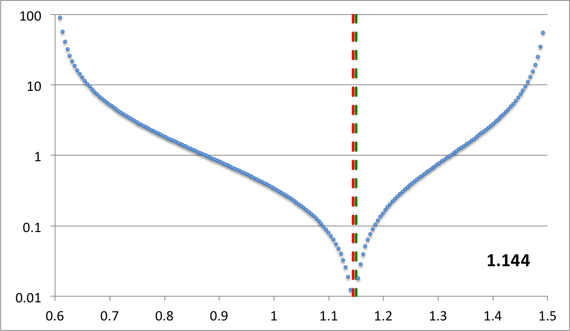
| |
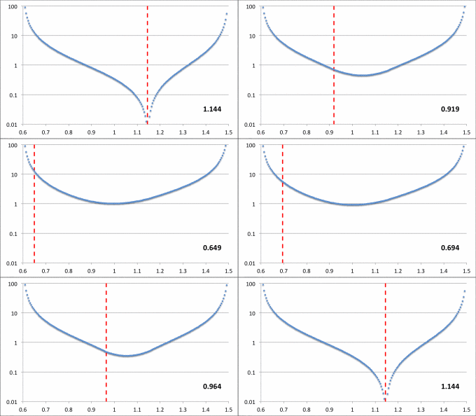 | |
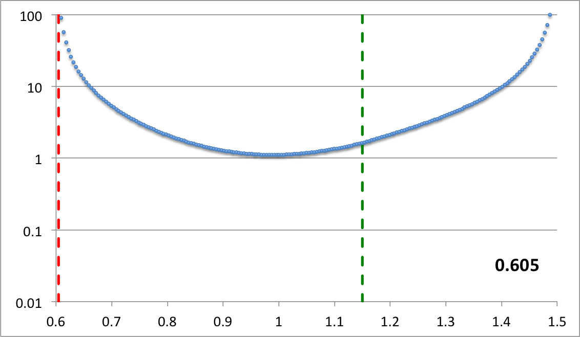 | |
|
Here we set <math>~r_- = 0.6</math>, <math>~r_+ = 1.5</math>, <math>~r_\mathrm{blue}= 1.15</math>, and <math>~p = 1.2</math>, then let the "green" edge vary over the range, <math>~0.605 \le r_\mathrm{green} \le 1.144</math>. Via an animation, the middle panel illustrates the behavior of our empirically constructed eigenfunction over this entire range of values as indicated by the numerical value shown in the bottom-righthand corner of the panel; the top and bottom panels display the shape of our eigenfunction at the two extreme values of <math>~r_\mathrm{green}</math>. |
|
Relationship to Fourier Series Amplitude and Phase
Recalling that,
|
<math>~e^{i\alpha}</math> |
<math>~=</math> |
<math>~\cos\alpha + i\sin\alpha \, ,</math> |
we appreciate that the real part of the amplitude term — the term inside the curly braces of the expression found in Figure 1, above — can be written as,
|
<math>~\mathcal{A}_m \equiv \Re\{f_m e^{im\phi}\}</math> |
<math>~=</math> |
<math>~f_m \cos(m\phi_m) \, .</math> |
When viewed in the context of a discrete Fourier series, we also recognize that the two functions, <math>~f_m</math> and <math>~\phi_m</math>, can be transformed into the pair of amplitude functions,
|
<math>~f_m ~~~\rightarrow ~~~ (a_m^2 + b_m^2)^{1/2}</math> |
and |
<math>~m\phi_m ~~~\rightarrow ~~~ \tan^{-1}\biggl(-\frac{b_m}{a_m}\biggr) \, ;</math> |
that is,
|
<math>~a_m ~=~ f_m\cos(m\phi_m)</math> |
and |
<math>~b_m ~=~ -f_m\sin(m\phi_m) \, .</math> |
Let's see where these expression lead us, given our above-adopted expressions for <math>~f_m</math> and <math>~\phi_m</math>. Given,
|
<math>~f = e^{f_\ln}</math> |
<math>~=</math> |
<math>~\biggl( \frac{r_\mathrm{blue} - \varpi}{\varpi - r_-} \biggr)^{p} \, ,</math> |
and,
|
<math>~m\phi_m</math> |
<math>~=</math> |
<math>~\tan^{-1}[\aleph \cdot D(\varpi)] \, </math> |
where,
|
<math>~D(\varpi)</math> |
<math>~=</math> |
<math>~\frac{f_\ln(\varpi) - [f_\ln]_\mathrm{min}}{[f_\ln]_\mathrm{max} - [f_\ln]_\mathrm{min}} \, ,</math> |
we have,
|
<math>~a_m</math> |
<math>~=</math> |
<math>~ \biggl( \frac{r_\mathrm{blue} - \varpi}{\varpi - r_-} \biggr)^{p} \cos\biggl[ \tan^{-1}\biggl( \aleph \cdot D \biggr) \biggr] </math> |
|
|
<math>~=</math> |
<math>~ e^{f_\ln} \biggl[ 1+(\aleph \cdot D )^2 \biggr]^{-1/2} </math> |
|
|
<math>~=</math> |
<math>~ e^{f_\ln} \bigg\{ 1+\aleph^2_\mathrm{norm} \biggl( f_\ln(\varpi) - [f_\ln]_\mathrm{min} \biggr)^2 \biggr\}^{-1/2} \, , </math> |
where,
<math>~\aleph_\mathrm{norm} \equiv \frac{\aleph}{[f_\ln]_\mathrm{max} - [f_\ln]_\mathrm{min}} \, .</math>
Another Improvement
I've realized that the phase plot is much smoother — in particular, the derivatives of both segments appear to match at their point of intersection — if we use <math>~D^{1/2}</math>, instead of simply <math>~D</math>, as the argument of the arctangent function. So, we define,
|
<math>~D_{1/2}(\varpi)</math> |
<math>~\equiv</math> |
<math>~\sqrt{D(\varpi)} = \biggl[ \frac{f_\ln(\varpi) - [f_\ln]_\mathrm{min}}{[f_\ln]_\mathrm{max} - [f_\ln]_\mathrm{min}} \biggr]^{1/2} \, ,</math> |
and henceforth will set,
|
With this new argument for the arctangent function, we have,
|
<math>~a_m</math> |
<math>~=</math> |
<math>~ \biggl( \frac{r_\mathrm{blue} - \varpi}{\varpi - r_-} \biggr)^{p} \cos\biggl[ \tan^{-1}\biggl( \aleph \cdot D_{1/2} \biggr) \biggr] </math> |
|
|
<math>~=</math> |
<math>~ e^{f_\ln} \biggl[ 1+(\aleph \cdot D_{1/2} )^2 \biggr]^{-1/2} </math> |
|
|
<math>~=</math> |
<math>~ e^{f_\ln} \bigg\{ 1+\aleph^2_\mathrm{norm} \biggl( f_\ln(\varpi) - [f_\ln]_\mathrm{min} \biggr) \biggr\}^{-1/2} </math> |
|
|
<math>~=</math> |
<math>~ e^{f_\ln} \bigg\{ C_0 +\aleph^2_\mathrm{norm} f_\ln(\varpi) \biggr\}^{-1/2} \, , </math> |
where,
<math>~C_0 \equiv 1 - \aleph_\mathrm{norm}^2 [f_\ln]_\mathrm{min} \, ,</math>
and,
<math>~\aleph_\mathrm{norm} \equiv \frac{\aleph^2}{[f_\ln]_\mathrm{max} - [f_\ln]_\mathrm{min}} \, .</math>
Specific Application to HI11's Figure 16
Next, let's see how well we can match the eigenmode structures presented in Figure 16 of HI11 by varying only a single parameter in our expression for <math>~f_\ln(\varpi)</math>. Given the radial locations of the inner and outer edges of the torus (normalized to the location of the density maximum; see the last two columns of our Table 1), <math>~r_- = 0.611</math> and <math>~r_+ = 1.490</math>, we set up an Excel spreadsheet with 199 radial zones spanning this range of radii.
| Table 1: HI11 Model Parameters | ||||||||
| Extracted from Table 2 of HI11 | Deduced Here | |||||||
| <math>~T/|W|</math> | <math>~n</math> | <math>~q</math> | <math>~R_\mathrm{max}</math> | <math>~R_+</math> | <math>~R_-/R_+</math> | <math>~\epsilon \equiv \frac{R_\mathrm{max}-R_-}{R_\mathrm{max}}</math> | <math>~r_- \equiv \frac{R_-}{R_\mathrm{max}}</math> | <math>~r_+ \equiv \frac{R_+}{R_\mathrm{max}}</math> |
| <math>~0.2729</math> | <math>~\tfrac{3}{2}</math> | <math>~\tfrac{3}{2}</math> | <math>~6.744</math> | <math>~10.051</math> | <math>~0.410</math> | <math>~0.388</math> | <math>~0.611</math> | <math>~1.490</math> |
Specifically, in Excel we set,
|
<math>~\delta r</math> |
<math>~=</math> |
<math>~\frac{r_+ - r_-}{200} = 0.004395 </math> |
|
<math>~$A$N</math> |
<math>~=</math> |
<math>~r_- + N \delta r</math> |
|
<math>~p</math> |
<math>~=</math> |
<math>~1.2 </math> |
Table 2 tabulates the value of <math>~f_\mathrm{blue}</math> over a range of radii for the specific case when we set <math>~r_\mathrm{blue} = 1.107635</math>.
|
Table 2:
Left-hand (blue) segment of eigenfunction |
|||
|
<math>~r_\mathrm{blue} = $A$113 = 1.107635</math> |
|||
| Example Excel Grid Zone | Function Evaluated | ||
| <math>~N</math> | <math>~\varpi</math> | <math>~f_\mathrm{blue}</math> | <math>~\ln(f_\mathrm{blue})</math> |
| 1 | 0.615395 | 287.78 | 5.6622 |
| 2 | 0.61979 | 123.92 | 4.8197 |
| 32 | 0.75164 | 3.04791 | 1.1145 |
| 50 | 0.83075 | 1.3195 | 0.27733 |
| 62 | 0.88349 | 0.79107 | -0.23437 |
| 82 | 0.97139 | 0.31121 | -1.1673 |
| 92 | 1.01534 | 0.16987 | -1.7727 |
| 102 | 1.05929 | 0.06908 | -2.6725 |
| 112 | 1.10324 | 0.003475 | -5.66220 |
Then, for two separate choices of <math>~r_\mathrm{green}</math> — specifically, 1.05929 and 0.61979 — Table 3 lists values of <math>~f_\mathrm{green}</math> at various radial positions across the HI11 torus. Given values of <math>~f_\mathrm{blue}</math> and <math>~f_\mathrm{green}</math> at each radial position, Table 3 also lists corresponding values of <math>~f_\ln</math>, <math>~D_{1/2}</math>, and <math>~\phi_1</math>. Notice that the values of <math>~[f_\ln]_\mathrm{min}</math> (highlighted in yellow) and <math>~[f_\ln]_\mathrm{max}</math> (highlighted in orange) that are used in the calculation of <math>~D_{1/2}</math> depend on the choice of <math>~r_\mathrm{green}</math>.
|
Table 3:
Right-hand (green) segment, and total eigenfunction |
||||||||
| <math>~r_\mathrm{green}</math> | Example Excel Grid Zone | Functions Evaluated† | ||||||
| <math>~N</math> | <math>~\varpi</math> | <math>~f_\mathrm{green}</math> | <math>~f_\mathrm{blue}</math> | <math>~f_\ln \equiv \ln(f_\mathrm{green}+f_\mathrm{blue})</math> | <math>~D_{1/2}</math> | <math>~(\phi_1/\pi)</math> | ||
|
<math>~$A$102 = 1.05929</math>
|
199 | 1.485605 | 242.17 | 0.0 | +5.490 | 0.9897 | -0.4212 | |
| 151 | 1.274645 | 1.00000 | 0.0 | 0.000 | 0.5750 | -0.3695 | ||
| 112 | 1.10324 | 0.073556 | 0.003475 | -2.564 | 0.1662 | -0.1868 | ||
| 106 | 1.07687 | 0.022632 | 0.038349 | -2.797 | <math>~\leftarrow~~[f_\ln]_\mathrm{min}</math> | 0.0000 | 0.0000 | |
| 103 | 1.063685 | 0.004129 | 0.060897 | -2.733 | 0.0871 | +0.1068 | ||
| 1 | 0.615395 | 0.0 | 287.78 | +5.662 | <math>~\leftarrow~~[f_\ln]_\mathrm{max}</math> | 1.0000 | +0.4220 | |
|
<math>~$A$2 = 0.61979</math>
|
199 | 1.485605 | 566.71 | 0.0 | +6.340 | <math>~\leftarrow~~[f_\ln]_\mathrm{max}</math> | 1.0000 | -0.4220 |
| 151 | 1.274645 | 3.79829 | 0.0 | +1.335 | 0.4673 | -0.3436 | ||
| 112 | 1.10324 | 1.30705 | 0.003475 | +0.270 | 0.2285 | -0.2357 | ||
| 106 | 1.07687 | 1.12898 | 0.038349 | +0.155 | 0.1848 | -0.2026 | ||
| 103 | 1.063685 | 1.04969 | 0.060897 | +0.105 | 0.1623 | -0.1833 | ||
| 83 | 0.975785 | 0.64322 | 0.29488 | -0.064 | <math>~\leftarrow~~[f_\ln]_\mathrm{min}</math> | 0.0000 | 0.0000 | |
| 1 | 0.615395 | 0.0 | 287.78 | +5.662 | 0.9456 | +0.4177 | ||
|
†Throughout this table, the phase angle, <math>~\phi_1(\varpi)</math>, has been calculated assuming that <math>~\aleph = 4</math>, and it has been assigned a positive (negative) value if <math>~\varpi</math> is inside (outside) the radial location (identified in red) of the minimum function value, <math>~[f_\ln]_\mathrm{min}</math>. |
||||||||
The miniaturized image displayed near the top of the left-most column of Table 3 contains a pair of plots associated with our choice of the parameter, <math>~r_\mathrm{green} = 1.05929</math>: On the left is a semi-log plot of the eigenfunction, <math>~f_\ln</math> versus <math>~\varpi</math> — actually, <math>~f_\mathrm{log10}</math> versus <math>~\varpi</math> — and on the right is a plot in polar coordinates of <math>~\phi_1</math> versus <math>~\varpi</math>, that is, a "constant phase locus" plot. In an analogous manner, the miniaturized image displayed near the bottom of the left-most column of Table 3 contains a semi-log plot of the radial eigenfunction and a polar plot of the "constant phase locus" associated with our choice of the parameter, <math>~r_\mathrm{green} = 0.61979</math>. The pair of plots found in each of these miniaturized images also appear within a single frame of the animation that is displayed in Figure 8, below. Each frame of the animation is stamped with the numerical value corresponding to the radial coordinate, <math>~r_\mathrm{min}</math>, at which the eigenfunction has its minimum (see the red numbers in Table 3). In the case of <math>~r_\mathrm{green} = 1.05929</math>, we find <math>~r_\mathrm{min} = 1.077</math>; and in the case of <math>~r_\mathrm{green} = 0.61979</math>, we find <math>~r_\mathrm{min} = 0.976</math>.
|
Figure 8: Radial and Azimuthal Eigenfunction Comparison |
||||||||||||||||||
| (a) Our Empirically Constructed Function | (b) Extracted from Figure 16 of HI11 | |||||||||||||||||
|
||||||||||||||||||
Material that appears after this point in our presentation is under development and therefore
may contain incorrect mathematical equations and/or physical misinterpretations.
| Go Home |
Attempts to Match P-modes and E-modes
Based especially on the analysis provided in Paper I and Paper II of the Imamura & Hadley collaboration, the eigenvectors that have drawn our attention thus far can be categorized as J-modes (as discussed, for example, in §3.2.1, Table 1 & Figure 2 of Paper II) or I-modes. Our empirically derived phase function needs to be altered in order to provide reasonable fits to the constant phase loci associated with P-modes and edge-modes (as discussed, for example in §3.2.2, Table2, Figures 3 & 4 of Paper II). We begin by constructing a table of equilibrium parameter values for the typical P- and E-mode models described in Table 2 of Paper II.
Setup
| Table 4: P- and E-mode Model Parameters Highlighted in Paper II K. Z. Hadley, P. Fernandez, J. N. Imamura, E. Keever, R. Tumblin, & W. Dumas (2014, Astrophysics and Space Science, 353, 191-222) | |||||||||
| Extracted from Table 2 or Table 4 of Paper II | Deduced Here | Extracted from Fig. 3 or Fig. 4 of Paper II | |||||||
| Name | <math>~M_*/M_d</math> | <math>~(n, q)</math>† | <math>~R_-/R_+</math> | <math>~r_\mathrm{outer} \equiv \frac{R_+}{R_\mathrm{max}}</math> | <math>~R_\mathrm{max}</math> | <math>~R_+</math> | <math>~\epsilon \equiv \frac{R_\mathrm{max}-R_-}{R_\mathrm{max}}</math> | <math>~r_- \equiv \frac{R_-}{R_\mathrm{max}}</math> | Eigenfunction |
| E1 | <math>~100</math> | <math>~(\tfrac{3}{2}, 2)</math> | <math>~0.101</math> | <math>~5.52</math> | <math>~0.00613</math> | <math>~0.0338</math> | <math>~0.442</math> | <math>~0.558</math> | |
| E2 | <math>~100</math> | <math>~(\tfrac{3}{2}, 2)</math> | <math>~0.202</math> | <math>~2.99</math> | <math>~0.0229</math> | <math>~0.0685</math> | <math>~0396</math> | <math>~0.604</math> | 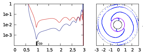 |
| E3 | <math>~100</math> | <math>~(\tfrac{3}{2}, 2)</math> | <math>~0.402</math> | <math>~1.74</math> | <math>~0.159</math> | <math>~0.277</math> | <math>~0.301</math> | <math>~0.699</math> | 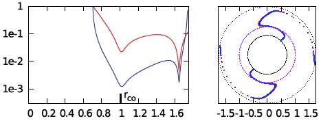 |
| P1 | <math>~100</math> | <math>~(\tfrac{3}{2}, 2)</math> | <math>~0.452</math> | <math>~1.60</math> | <math>~0.254</math> | <math>~0.406</math> | <math>~0.277</math> | <math>~0.723</math> | 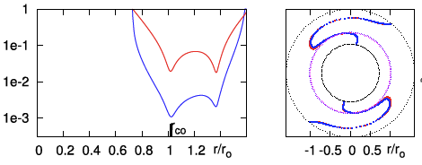 |
| P2 | <math>~100</math> | <math>~(\tfrac{3}{2}, 2)</math> | <math>~0.500</math> | <math>~1.49</math> | <math>~0.403</math> | <math>~0.600</math> | <math>~0.255</math> | <math>~0.745</math> | 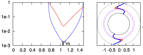 |
| P3 | <math>~100</math> | <math>~(\tfrac{3}{2}, 2)</math> | <math>~0.600</math> | <math>~1.33</math> | <math>~1.09</math> | <math>~1.450</math> | <math>~0.202</math> | <math>~0.798</math> | |
| P4 | <math>~100</math> | <math>~(\tfrac{3}{2}, 2)</math> | <math>~0.700</math> | <math>~1.21</math> | <math>~3.37</math> | <math>~4.078</math> | <math>~0.153</math> | <math>~0.847</math> | |
| †In all three papers from the Imamura & Hadley collaboration, <math>~q = 2</math> means, "uniform specific angular momentum." | |||||||||
As in our separate summary discussion, our two-piece radial eigenfunction is defined by the expressions,
|
<math>~f_\mathrm{blue}(\varpi) </math> |
<math>~=</math> |
<math>~\biggl( \frac{r_\mathrm{blue} - \varpi}{\varpi - r_-} \biggr)^{p} </math> |
for |
<math>r_- < \varpi < r_\mathrm{blue} </math> … <math>~\biggl[ f_\mathrm{blue}(\varpi) = 0</math> otherwise<math>~\biggr]</math>, |
and,
|
<math>~f_\mathrm{green}(\varpi) </math> |
<math>~=</math> |
<math>~\biggl( \frac{r_\mathrm{green} - \varpi}{\varpi - r_+} \biggr)^{p} </math> |
for |
<math>r_\mathrm{green} < \varpi < r_+ </math> … <math>~\biggl[ f_\mathrm{green}(\varpi) = 0</math> otherwise<math>~\biggr]</math>, |
where, <math>~r_\mathrm{mid}|_\mathrm{green} \le r_\mathrm{mid}|_\mathrm{blue}</math>. The expression that we are currently using for the radial eigenfunction is a sum of these two pieces, that is,
|
Over the inner ("blue") region of the torus, we will continue to use the phase-function prescription that has been described in our separate summary discussion, namely,
|
where, <math>~\aleph_m</math> is a constant,
|
<math>~D_{1/2}(\varpi)</math> |
<math>~\equiv</math> |
<math>~\biggl[ \frac{f_\ln(\varpi) - [f_\ln]_\mathrm{min}}{[f_\ln]_\mathrm{max} - [f_\ln]_\mathrm{min}} \biggr]^{1/2} \, ,</math> |
|
<math>~f_\ln(\varpi)</math> |
<math>~\equiv</math> |
<math>~\ln[ f_1(\varpi)] \, .</math> |
and, <math>~r_\mathrm{min}</math> is the radial location of the minimum of the radial eigenfunction, <math>~f_\ln</math>. Over the outer ("green") region of the torus, however, we now adopt a different prescription for the phase function, namely,
|
where, <math>~A_0</math> is a constant.
Application to Specific Models
In what follows, we pick a model from Table 4, and extract from that model the locations of the inner and outer radii of the torus, namely, <math>~r_-</math> and <math>~r_\mathrm{outer}</math>. Then, in an effort to construct an eigenvector that matches the behavior shown in the corresponding Paper II plots (as reprinted, here, in the last column of our Table 4) over the innermost region of the configuration — that is, the region around the innermost and most prominent minimum of the radial eigenfunction — we assign a value to <math>~r_\mathrm{blue}</math> that roughly corresponds to the radial location of the first (innermost) minimum, and we assign a value to <math>~r_+</math> that roughly corresponds to the radial location of the second minimum. We set <math>~m = 2</math> for each model, because, following Hadley et al. (2014), we are focusing only on unstable P- and E-modes having "bar-like" structures; and, as above, when descritizing each model within Excel, we set,
|
<math>~\delta r</math> |
<math>~=</math> |
<math>~\frac{r_+ - r_-}{200} </math> |
|
<math>~$A$N</math> |
<math>~=</math> |
<math>~r_- + N \delta r \, .</math> |
Then, for each model, we adjusted the values of five free parameters until a reasonably good fit to both the published radial eigenfunction and "constant phase locus" was obtained over the innermost region of the model. The five adjustable parameters are: <math>~p_\mathrm{blue}, ~r_\mathrm{green}, ~p_\mathrm{green}, ~\aleph_2,</math> and <math>~A_0</math>.
| Table 5: Model E2‡ | ||||
| Model Parameters | Results from Paper II (Hadley et al. 2014) Simulation | |||
| <math>~r_-</math> | <math>~r_+</math> | <math>~r_\mathrm{outer}</math> | <math>~\delta r</math> | |
| <math>~0.60</math> | <math>~2.0</math> | <math>~3.0</math> | <math>~0.007</math> | |
| <math>~r_\mathrm{blue}</math> | <math>~p_\mathrm{blue}</math> | <math>~r_\mathrm{green}</math> | <math>~p_\mathrm{green}</math> | |
| <math>~$A$68 = 1.006</math> | <math>~1.2</math> | <math>~$A$65 = 0.985</math> | <math>~0.50</math> | |
| <math>~r_\mathrm{min}</math> | <math>~[f_\ln]_\mathrm{min}</math> | <math>~[f_\ln]_\mathrm{max}</math> | Our Empirically Constructed Eigenvector | |
| <math>~$A$65 = 0.985</math> | <math>~-3.49047</math> | <math>~\ln[f_2($A$1)]=+4.85166</math> | ||
| <math>~m</math> | <math>~\aleph_2</math> | <math>~A_0</math> | <math>~\phi_0</math> | |
| <math>~2</math> | <math>~\pi</math> | <math>~0.25</math> | <math>~\tfrac{9\pi}{16}</math> | |
|
‡Note the following:
|
||||
| Table 6: Model E3‡ | ||||
| Model Parameters | Results from Paper II (Hadley et al. 2014) Simulation | |||
| <math>~r_-</math> | <math>~r_+</math> | <math>~r_\mathrm{outer}</math> | <math>~\delta r</math> | |
| <math>~0.7</math> | <math>~1.7</math> | <math>~1.74</math> | <math>~0.005</math> | |
| <math>~r_\mathrm{blue}</math> | <math>~p_\mathrm{blue}</math> | <math>~r_\mathrm{green}</math> | <math>~p_\mathrm{green}</math> | |
| <math>~$A$77 = 1.085</math> | <math>~1.2</math> | <math>~$A$55 = 0.975</math> | <math>~0.75</math> | |
| <math>~r_\mathrm{min}</math> | <math>~[f_\ln]_\mathrm{min}</math> | <math>~[f_\ln]_\mathrm{max}</math> | Our Empirically Constructed Eigenvector | |
| <math>~$A$71 = 1.055</math> | <math>~-1.34494</math> | <math>~\ln[f_2($A$1)]=+5.19688</math> | ||
| <math>~m</math> | <math>~\aleph_2</math> | <math>~A_0</math> | <math>~\phi_0</math> | |
| <math>~2</math> | <math>~\tfrac{11 \pi}{8}</math> | <math>~3.0</math> | <math>~\tfrac{2\pi}{5}</math> | |
|
‡Note the following:
|
||||
| Table 7: Model P1‡ | ||||
| Model Parameters | Results from Paper II (Hadley et al. 2014) Simulation | |||
| <math>~r_-</math> | <math>~r_+</math> | <math>~r_\mathrm{outer}</math> | <math>~\delta r</math> | |
| <math>~0.723</math> | <math>~1.35</math> | <math>~1.6</math> | <math>~0.003135</math> | |
| <math>~r_\mathrm{blue}</math> | <math>~p_\mathrm{blue}</math> | <math>~r_\mathrm{green}</math> | <math>~p_\mathrm{green}</math> | |
| <math>~$A$100 = 1.00515</math> | <math>~1.0</math> | <math>~$A$96 = 0.99261</math> | <math>~0.35</math> | |
| <math>~r_\mathrm{min}</math> | <math>~[f_\ln]_\mathrm{min}</math> | <math>~[f_\ln]_\mathrm{max}</math> | Our Empirically Constructed Eigenvector | |
| <math>~$A$96 = 0.99261</math> | <math>~-3.06805</math> | <math>~\ln[f_2($A$1)]=+4.48864</math> | ||
| <math>~m</math> | <math>~\aleph_2</math> | <math>~A_0</math> | <math>~\phi_0</math> | |
| <math>~2</math> | <math>~2.55</math> | <math>~0.094</math> | <math>~\tfrac{\pi}{2}</math> | |
|
‡Note the following:
|
||||
See Also
- Imamura & Hadley collaboration:
- Paper I: K. Hadley & J. N. Imamura (2011, Astrophysics and Space Science, 334, 1-26), "Nonaxisymmetric instabilities in self-gravitating disks. I. Toroids" — In this paper, Hadley & Imamura perform linear stability analyses on fully self-gravitating toroids; that is, there is no central point-like stellar object and, hence, <math>~M_*/M_d = 0.0</math>.
- Paper II: K. Z. Hadley, P. Fernandez, J. N. Imamura, E. Keever, R. Tumblin, & W. Dumas (2014, Astrophysics and Space Science, 353, 191-222), "Nonaxisymmetric instabilities in self-gravitating disks. II. Linear and quasi-linear analyses" — In this paper, the Imamura & Hadley collaboration performs "an extensive study of nonaxisymmetric global instabilities in thick, self-gravitating star-disk systems creating a large catalog of star/disk systems … for star masses of <math>~0.0 \le M_*/M_d \le 10^3</math> and inner to outer edge aspect ratios of <math>~0.1 < r_-/r_+ < 0.75</math>."
- Paper III: K. Z. Hadley, W. Dumas, J. N. Imamura, E. Keever, & R. Tumblin (2015, Astrophysics and Space Science, 359, article id. 10, 23 pp.), "Nonaxisymmetric instabilities in self-gravitating disks. III. Angular momentum transport" — In this paper, the Imamura & Hadley collaboration carries out nonlinear simulations of nonaxisymmetric instabilities found in self-gravitating star/disk systems and compares these results with the linear and quasi-linear modeling results presented in Papers I and II.

|
|---|
|
© 2014 - 2021 by Joel E. Tohline |

